A Comprehensive Mechanistic Interpretability Explainer & Glossary
The main doc is hosted on Dynalist, which has a much better UI for long docs and I highly recommend reading it there. The below is a janky HTML dump for those who prefer this UI
Introduction
- Why does this doc exist?
- The goal of this doc is to be a comprehensive glossary and explainer for Mechanistic Interpretability (focusing on transformer language models), the field of studying how to reverse engineer neural networks.
- There's a lot of complex terms and jargon in the field! And these are often scattered across various papers, which tend to be pretty well-written but not designed to be an introduction to the field as a whole. The goal of this doc is to resolve some research debt and strives to be a canonical source for explaining concepts in the field
- I try to go beyond just being a reference that gives definitions, and to actually dig into how to think about a concept. Why does it matter? Why should you care about it? What are the subtle implications and traps to bear in mind? What is the underlying intuition, and how it fits into the rest of the field?
- I also go outside pure mechanistic interpretability, and try to define what I see as the key terms in deep learning and in transformers, and how I think about them. If you want to reverse engineer a system, it's extremely useful to have a deep model of what's going on inside of it. What are the key components and moving parts, how do they fit together, and how could the model use them to express different algorithms?
- How to read this doc?
- The first intended way is to use this a reference. When reading papers, or otherwise exploring and learning about the field, coming here and looking up any terms and trying to understand them.
- The second intended way is to treat this as a map to the field. My hope is that if you're new to the field, you can just read through this doc from the top, get introduced to the key ideas, and be able to dig into further sources when confused. And by the end of this, have a pretty good understanding of the key ideas, concepts and results!
- It's obviously not practical to fully explain all concepts from scratch! Where possible, I link to sources that give a deeper explanation of an idea, or to learn more.
- More generally, if something’s not in this glossary, you can often find something good by googling it or searching on alignmentforum.org. If you can’t, let me know!
- I frequently go on long tangents giving my favourite intuitions and context behind a concept - it is not at all necessary to understand these (though hopefully useful!), and I recommend moving on if you get confused and skimming these if you feel bored.
- Why does this doc exist?
Mechanistic Interpretability
Key concepts and terms in mechanistic interpretabilityGeneral
Basic ideas, like a features and circuit, and the surrounding intuitions and how best to think about them- MI/mech int/mech interp/mechanistic interpretability: The field of study of reverse engineering neural networks from the learned weights down to human-interpretable algorithms. Analogous to reverse engineering a compiled program binary back to source code
- Interpretability: The broader subfield of AI studying why AI systems do what they do, and trying to put this into human-understandable terms.
- There isn’t a clear consensus on exactly what interpretability is about, what the goals of the field are, the right standards of and types of evidence, etc.
- The Mythos of Model Interpretability and Towards A Rigorous Science of Interpretable Machine Learning are good attempts to disentangle this.
- See The Broader Interpretability Field for more discussion of this, and how MI differs from/overlaps with the broader field.
- There isn’t a clear consensus on exactly what interpretability is about, what the goals of the field are, the right standards of and types of evidence, etc.
- A feature is a property of an input to the model, or some subset of that input (eg a token in the prompt given to a language model, or a patch of an image)
- This is a fuzzy and non-rigorous idea, best illustrated by examples:
- This part of the image contains a curve
- This is a feature in a convnet, where there’s a neuron activation per image patch - thus “part of image”
- This part of the image contains a dog fur-like texture
- This token is the final token in the phrase “Eiffel Tower”
- In a factual recall circuit, this can get looked up to produce the feature “is in Paris”
- This is a feature in a transformer, where there are separate activations for each token in a sequence, thus “this token”
- This text is Python code
- This token is the name of a variable corresponding to a list in Python code
- This token is in a news headline in a Reuters article
- This token corresponds to a number that is being used to describe a group of people
- This text is a Bible verse
- This text is an excerpt from Harry Potter
- This part of the image contains a curve
- Implicit fuzzy things about how the term is used in practice:
- This is normally used to describe a property of an example input that is actually internally represented in the model, rather than a feature that could be in theory.
- It’s used to refer to properties of inputs that generalise across inputs, eg “is this a dog” rather than “is this the specific picture that appeared in the training data”
- Often used interchangeably with the more specific term interpretable features
- It’s somewhat fuzzy whether you can have a feature that is not interpretable. An edge case is described in Adversarial Examples are Features Not Bugs, where they find that adversarial examples seem to pick up on subtle features in images that humans can’t detect, but which have predictive power and transfer to images that were not trained on - it’s not obvious to me whether these count as interpretable or not.
- This is a fuzzy and non-rigorous idea, best illustrated by examples:
- Features are the fundamental building block of models - the model’s internal activations represent features, and the model’s weights and non-linearities are used to apply computations to produce later features from earlier features. The subset of a model’s weights and non-linearities used to map a set of earlier features to a set of later features is called a circuit
- Circuit is also a fairly fuzzy and poorly defined term. Intuitively, a circuit means “the sub part of a model that does some understandable computation to produce some interpretable features from prior interpretable features”. A special case is when some of the features are the inputs or the outputs, which are inherently interpretable (hopefully!). Ideally, the intermediate steps of computation also represent interpretable features, but this is not essential.
- Examples of well understood circuits: (All described in more detail later)
- Curve circuits: A circuit in inception that identifies which parts of an image contain curves (with a separate neuron for each curve orientation)
- Induction circuits: A circuit in generative language models that involves two attention heads (a previous token head and an induction head) composing to detect and continue repeated subsequences.
- The Indirect Object Identification Circuit (IOI): A circuit used to complete the sentence “John and Mary went to the shops, then John gave a bottle of milk to” with “ Mary” not “ John”
- Examples of well understood circuits: (All described in more detail later)
- Circuit is also a fairly fuzzy and poorly defined term. Intuitively, a circuit means “the sub part of a model that does some understandable computation to produce some interpretable features from prior interpretable features”. A special case is when some of the features are the inputs or the outputs, which are inherently interpretable (hopefully!). Ideally, the intermediate steps of computation also represent interpretable features, but this is not essential.
- A special case is an end-to-end circuit, where the circuit describes how the input to the model is converted to the output (ideally with several interpretable intermediate computations).
- Induction heads and Indirect Object Identification are end-to-end circuits, curve circuits are not (because the output of a circuit curve is a neuron that represents that curve orientation)
- Intervening on or editing an activation means to run the network, then to stop it once it’s computed an activation, edit or replace that activation, and then resume running the model with the edited activation replacing the old one.
- An example intervention is pruning. Pruning a neuron means to intervene on the neuron’s activation and set it to zero, so later layers in the model cannot use that neuron’s output.
- Equivariance / Neuron families: When there is a family of neurons or features that are distinct but analogous, and where we expect understanding of one to translate to understanding of the others.
- Eg neurons that detect lines or curves of different orientations, or neurons that detect whether the token “ die” is in English, German or Dutch text
- Neuron splitting: Where a feature in one model gets decomposed into several features in a larger model.
- Eg “a character in hexadecimal” -> “the character 3 in hexadecimal” (and for the other 15 characters!)
- Universality: The hypothesis that the same circuits will show up in different models.
- This is a somewhat fuzzy concept - my interpretation is the idea that there is some “best” or “correct” way to complete some task on some data distribution in some model architecture, and that different models trained to do similar tasks on similar data with similar architectures are likely to converge on it.
- The bolder (and IMO probably false) hypothesis is that circuits represent some deep principles of how neural networks learn, that there is some finite (and hopefully not too large!) family of important circuits to understand, and that we can characterise eg language model training by seeing which circuits develop at which points in training.
- Motif: A fuzzy notion of some abstract notion that recurs between circuits or features in different models/contexts
- Neuron splitting and equivariance are one example
- Attention heads composing to form induction heads are another example
- Induction heads themselves are an example, as they seem to underlie more complex behaviour like translation and few-shot learning
- A model behaviour is localised or sparse when it is determined by only a few components in the model.
- Eg, the behaviour of predicting the next token in a repeated subsequence can be localised to the previous token head and induction head.
- This is again a fuzzy notion:
- Model behaviour can mean many things (why does a head look here? Why does this neuron activate? Why does the model get high loss on this task?).
- It can also be relative to some default behaviour. Eg, in the IOI task ”why does it have a higher indirect object logit then the subject logit?” tracks the fact that the model predicts the indirect object more than the subject, given that it predicts a name that occurred earlier in the sentence at all, but doesn’t eg check whether it predicts a word like “ the” higher than either name.
- “Determined by” is also fuzzy - normally almost all parts of the model contribute a bit, but some contribute far more than others. See causal scrubbing for an attempt to operationalise this.
- Model behaviour can mean many things (why does a head look here? Why does this neuron activate? Why does the model get high loss on this task?).
- Localisation matters because it makes model behaviour much easier to reverse engineer, and suggests that there is some legible circuit to be understood.
- In practice, a surprising amount of behaviours are localised, but many are not! Often careful setups of the task and behaviour in question and what is being controlled for can help.
- Microscope AI is the idea that, if we train a superhuman model, rather than needing to use it (with all of the associated dangers), we could instead reverse engineer it, learn what it has learned about the world, and use this knowledge ourselves.
- I don’t think it’s particularly practical, but it’s a nice aspiration for what a world with amazing mechanistic interpretability could look like!
Representations of Features & Superposition
How should we think about the way features are represented in the model- The curse of dimensionality is the idea that things can get weird and confusing when examining high-dimensional systems (relative to low-dimensional systems)
- Specifically in mechanistic interpretability, the problem is that neural network activations live in a very high dimensional space, and the weights lie in an even higher dimensional space. This is basically impossible to understand intrinsically, so we need a way to break the high-dimensional object down into lower dimensional pieces that can be understood independently-ish.
- The main way of doing this is to find a way of decomposing the model’s internal activations into features, and using this to decompose the weights into circuits connecting up features. Obviously, we need to be careful to do this in a way that is principled and actually true to the ground truth of the model, and not just projecting what we want to be true!
- Key properties of features and their representation inside the model:
- They should be able to vary semi-independently (though are likely correlated/anti-correlated)
- The features are useful for computing the model’s output (ie, there is mutual information between that feature and the correct output).
- The features can be recovered from the model’s activations, ideally with linear operations like projections (since most of a model’s operations are matrix multiplies with learned weights)
- Features as directions is the hypothesis that features are represented in the model as directions in activation space.
- The intuition behind this is that the main thing a model is capable of doing is linear algebra - addition and matrix multiplication, which further breaks down into addition, scalar multiplication, and projecting onto specific directions. Given these capabilities, features as directions is an extremely natural way to represent things - if a later layer wants to access a feature it can project onto that feature’s direction, a neuron can easily access and combine multiple features, features can vary independently, and the component in that feature direction represents the strength of that feature.
- Note that this is a much more specific claim than the fuzzy notion that “model’s internal activations represent features”. I would say that the broader claim means that there is some function that can recover the features from these activations, even if we don’t know what that function is, and even if there’s no way to do this without a bunch of noise.
- If, specifically, features are directions in activation space, then the function to recover a feature from activations would be projecting onto that feature’s direction. Ideally the feature directions would be orthogonal, so that they can be perfectly recovered with a projection.
- Note that in this section I am trying to emphasise what representations the model is likely to find useful, rather than what I want it to do. See superposition for discussions of limitations of this framework.
- Implicit in the description of features as directions is that the feature can be represented as a scalar, and that the model cares about the range of this number. That is, it matters whether the feature
- This is an important and confusing point, and it’s worth digging into.
- Overly technical aside: Implicit in this is the idea that a model cares about the range of values that its representation of a feature takes on. It wants to represent the feature as a direction, and to apply linear maps to that, and so it wants to preserve the magnitude of that feature.
- This is in contrast to a purely binary feature, which is either true or false about an input.
- This may still be represented as a direction, but in practice the model just cares about whether that point in space is there, rather than the size of a component in a direction. Given that a model’s core operation is matrix multiplication, it’s not clear to me how much it’s worth representing a binary feature as a direction, vs compressing things together much more.
- Eg, “if the component in this direction is 0.4 it’s feature A, 0.6 it’s Feature B, and 1.0 it’s feature C” is a much cheaper way to represent binary features.
- In practice, this is a pretty imprecise description. Most features will be binary(-ish), but the model’s ability to tell will often be much more continuous, and involve weighing up evidence.
- A better phrasing might be whether the feature is bimodal (ie, it’s pretty obvious whether it’s true or false, and very few inputs are ambiguous), vs something that’s more uncertain with many ambiguous examples.
- Eg A feature like “is the current token the” or “is this computer code vs a romance novel” will be pretty obvious and binary, and the model likely won’t care about the magnitude.
- But for more complex questions (eg, the next word is a female vs male pronoun), the model will likely do a significant amount of weighing up and evaluating evidence, and will care about tracking exactly how confident it is.
- Continuous features: Features that lie on a spectrum, where they can be more or less present for an input.
- Eg, this is an image of water
- And, implicitly, where it matters how present they are, rather than being boring.
- This is in contrast to a purely binary feature, which is either true or false about an input.
- An interpretable basis is a set of directions in activation space where each direction corresponds to some interpretable feature.
- In the weak sense, this means a set of directions where we expect each to be an interpretable feature, but we don’t necessarily know what it is. In the strong sense, we have that and we know what all of the features are!
- For any activation in the model, the standard or canonical basis is the basis by which that activation is represented internally in the computer (and in the code) as a tensor of floats.
- A key example is neuron activations after a non-linearity - if there are n neurons, their activations is a direction in R^n. R^n is the activation space, and each neuron is a direction. We call the basis given by neuron directions the standard basis.
- A privileged basis is a meaningful basis for a vector space. That is, the coordinates in that basis have some meaning, that coordinates in an arbitrary basis do not have. It does not, necessarily, mean that this is an interpretable basis.
- Note that a space can have an interpretable basis without having a privileged basis. In order to be privileged, a basis needs to be interpretable a priori - ie we can predict it solely from the structure of the network architecture.
- Eg It is possible that we could infer an interpretable basis from the weights of the model with a dimensionality reduction technique (like SVD), but that if we retrained the model this technique would give a totally different interpretable basis.
- This is a useful distinction, because if we can identify a privileged basis and have reason to think that it’s (weakly) interpretable, then we can directly decompose the model’s activations into interpretable features.
- The main important example of a privileged basis is the basis of neuron directions immediately after an elementwise non-linearity, like ReLU or GELU. (ie the standard basis of neuron activation space) - in the standard basis a ReLU acts on each coordinate independently, but if we change basis then ReLU now affects ranges of coordinates in a weird and confusing way.
- This is a confusing concept, because we tend to focus on privileged bases, but actually all bases are non-privileged by default - vector spaces are a geometric object, and there’s no intrinsic meaning to any particular basis. We need a reason to think that a basis is privileged (like a ReLU).
- Another framing - if we’re only doing linear algebra, then there’s no such thing as a privileged basis. Operations like addition, matrix multiplication, dot products, etc are unchanged under any change of basis. So we need to look for a special non-linear operation affecting that vector space that might give it a privileged basis.
- Caveat: Technically, privileged/non-privileged bases is a somewhat leaky abstraction, and the standard basis is always slightly privileged. Floating point representations and Adam inherently privilege the standard basis, and are not the same under rotation. I mostly think of it as a spectrum from privileged to not privileged than a binary.
- Note that a space can have an interpretable basis without having a privileged basis. In order to be privileged, a basis needs to be interpretable a priori - ie we can predict it solely from the structure of the network architecture.
- A bottleneck activation/dimension is an intermediate activation in a low dimensional space between a map from a larger space and a map to a larger space.
- Most activations in a transformer are bottleneck dimensions: the residual stream, keys, queries and values. (I don’t believe that any activations in Inceptionv1 are bottlenecks?)
- The residual stream is subtle - it’s not the intermediate activation between a single map in and a single map out, but instead many layers read and write from it, but each operation is purely linear. Not all of these spaces have a higher dimension, but in aggregate many more dimensions go in than come out.
- Importantly, there are no non-linearities involved, so the bottleneck activation has no privileged basis (ish) - all spaces have no privileged basis by default!
- Intuition: It’s often useful to think about it as an intermediate step when multiplying by a low-rank factorization of a bigger matrix.
- Most activations in a transformer are bottleneck dimensions: the residual stream, keys, queries and values. (I don’t believe that any activations in Inceptionv1 are bottlenecks?)
- Features as neurons is the more specific hypothesis that, not only do features correspond to directions, but that each neuron corresponds to a feature, and that the neuron’s activation is the strength of that feature on that input.
- Aka, the standard basis of neuron activations is interpretable.
- Importantly, this is not obvious, and probably not entirely true! The only reason this is even somewhat plausible is that neuron activations.
- There is a decent amount of empirical evidence that this is mostly true of Inceptionv1, but this seems at best only slightly true for transformers.
- Check out a bunch of interpretable neurons in CLIP!
- Note: In a convnet, every activation space is immediately after a ReLU, so this describes every activation. In a transformer it’s somewhat more complicated - this only describes the internal activation space of an MLP layer, and not the residual stream.
- Enumerative safety is the (ambitious!) idea that we could reach a point where we understand every feature in the model, and could check through all of these to look for undesirable behaviour, eg deception
- The curse of dimensionality is the idea that things can get weird and confusing when examining high-dimensional systems (relative to low-dimensional systems)
Toy Model of Superposition
How to think about superposition, and concepts from A Toy Model of Superposition- Superpositionis when a model represents more than n features in an n dimensional activation space. That is, features still correspond to directions, but the set of interpretable directions is larger than the number of dimensions.
- This set of >n directions is sometimes called an overcomplete basis. (Notably, this is not a basis, because it is not linearly independent)
- A key consequence is that if superposition is being used, there cannot be an interpretable basis. In particular, features as neurons cannot perfectly hold.
- Sparse coding is a field of maths that finds techniques to find an overcomplete basis for a set of vectors such that each vector is a sparse linear combination of these basis vectors.
- Importantly, if we try to read each feature vs projecting onto some direction, these cannot all be orthogonal, so we cannot perfectly recover each feature.
- Equivalently, because any set of >n directions is not linearly independent, any activation can be written as infinitely many different linear combination of those directions, and so can’t be uniquely interpreted as a set of features.
- There are two kinds of superposition worth caring about in a transformer: (terms invented by me)
- Bottleneck dimension superposition - this is when a bottleneck dimension experiences superposition. (Eg keys, queries, the residual stream, etc)
- This is not very surprising! If there’s 50,000 tokens in the vocabulary and 768 dimensions in the residual stream, there almost has to be more features than dimensions, and thus superposition.
- Intuitively, bottleneck superposition is just used for “storage”, bottleneck dimensions are intermediate states of linear maps and we do not expect them to be doing significant computation.
- Neuron superposition - this is when neuron activations experience superposition. Ie, there are more features represented in neuron activation space than there are neurons.
- Intuitively, neuron superposition represents doing “computation” in superposition - using n non-linearities to perform computation for more than n features.
- Intuitively, bottleneck superposition is easier than neuron superposition - the only interference to care about is when projecting onto a feature direction is other features with non-zero dot product with that direction. While in neuron superposition, if one neuron has significant contribution from multiple features, then if one of those feature changes then that will affect all the other features in a weird and messy way.
- Is this actually harder to deal with in practice for a model? I have no idea! This is a pretty open question.
- Bottleneck dimension superposition - this is when a bottleneck dimension experiences superposition. (Eg keys, queries, the residual stream, etc)
- This set of >n directions is sometimes called an overcomplete basis. (Notably, this is not a basis, because it is not linearly independent)
- Neuron polysemanticity is the idea that a single neuron activation corresponds to multiple features. Empirically we might observe that, a neuron activates on multiple clusters of seemingly unrelated things like pictures of dice and pictures of poets.
- Subtlety: Neuron superposition implies polysemanticity (since there are more features than neurons), but not the other way round. There could be an interpretable basis of features, just not the standard basis - this creates polysemanticity but not superposition.
- Alternately, neuron polysemanticity is equivalent to saying that the standard basis is not interpretable.
- Conversely, a neuron is monosemantic if it corresponds to a single feature.
- In practice, the standards for calling a neuron monosemantic are somewhat fuzzy and it’s not a binary - if a neuron activates really strongly for a single feature, but activates a bit on a bunch of of other features, I’d probably call it monosemantic.
- We can both use polysemanticity to refer to the neuron layer as a whole, or to refer to a specific neuron as being polysemantic. A layer of neurons could contain both polysemantic and monosemantic neurons.
- Note: Polysemanticity isn’t used to refer to bottleneck dimensions, because there’s no privileged basis to be polysemantic in.
- Subtlety: Neuron superposition implies polysemanticity (since there are more features than neurons), but not the other way round. There could be an interpretable basis of features, just not the standard basis - this creates polysemanticity but not superposition.
- Anthropic’s Toy Model of Superposition paper gives a conceptual framework for thinking about superposition and features:
- Intuitively, superposition is a form of lossy compression. The model is able to represent more features, but at the cost of adding noise and interference between features. Models need to find an optimal point balancing between the two, and it’s plausible that the optimal point will not be zero superposition.
- There are two key aspects of a feature:
- Its importance - how useful is it for achieving lower loss? Important features are more useful to represent, and interference with them is more expensive
- Its sparsity - how frequently is it in the input? Controlling for importance, if a feature is sparse it will interfere with other features less.
- In general, problems with many sparse, unimportant features will show significant superposition.
- Superposed features of uniform importance tend to cluster in geometric configurations, where features cluster into subspaces, where each cluster lies in orthogonal subspaces but are in superposition within that cluster. If clusters form multiple orthogonal subspaces, these subspaces are said to be in a tegum product. (See Adam Jermyn’s post for some intuition on why this happens).
- Eg if four features are in a cluster in a 3D subspace, it can form a tetrahedron.
- Does this generalise to real models? Extremely unclear!
- A key geometric configuration is that of antipodal pairs. That is, a single direction, which represents feature 1 in the positive direction and feature 2 in the negative direction. I would guess this is the most likely configuration to generalise.
- A key observation is that (with ReLUs) antipodal pairs work totally fine if at most one of feature 1 and feature 2 is present, but breaks if both are. If both are sparse, this is totally fine - if they’re there 1% of the time, then this is useful 2% of the time and terrible 0.01% of the time.
- Correlated features will interfere more and tend to be more orthogonal, while anti-correlated features will interfere less and tend to be within the same tegum product.
- There’s some evidence that correlated features may form local almost-orthogonal bases - that is, if we take the subset of features that are pairwise correlated, because the model wants low interference, these correspond to orthogonal-ish directions that can be interpreted, even if features outside that set will interfere significantly.
- The paper mostly focuses on bottleneck superposition, but has some fascinating results on neuron superposition - in particular, finding the asymmetric superposition motif. (I’m not happy with this explanation - go check out the paper!)
- Rather than having “symmetric” superposition, where the two features interfere equally, the model has asymmetric superposition, where feature 1 interferes much more with feature 2 than vice versa.
- It then uses a separate neuron to clean up the interference, where the presence of feature 1 suppresses any impact of that neuron on the output for feature 2.
- Ie, if we have both feature 1 and feature 2, the neuron just thinks it has feature 1 - feature 1 has a much larger coefficient than feature 2.
- An underlying concept is that of the feature importance curve. There is, in theory, an arbitrary amount of features that matter, with a long tail of increasingly niche and unimportant features (like whether text occurs in a glossary about mechanistic interpretability!) which are still better than nothing. We can imagine enumerating all of these features, and then ordering them in decreasing order of importance. We’ll begin with incredibly important and frequent features (eg, “this is a new article” or “this is Python code”), and steadily drop off. Under this framing, we should expect models to always want to do non-zero superposition, as there will always be some incredibly sparse but useful feature it will want to learn (which may be extremely hard to detect!)
- Superpositionis when a model represents more than n features in an n dimensional activation space. That is, features still correspond to directions, but the set of interpretable directions is larger than the number of dimensions.
The Broader Interpretability Field
A brief attempt to position Mechanistic Interpretability in the context of the field of AI interpretability- An attempt to outline the field of interpretability to put MI in context. Note that I am both biased and much better placed to speak about MI than interpretability as a whole! Take the below with a pinch of salt
- Black-box interpretability: Studies the model as a black box mapping inputs to outputs, and tries to interpret it.
- Sometimes uses the fact that the model is differentiable to produce interpretations of the input (eg saliency maps), but is more focused on explaining the model’s behaviour than exploring the internals and what they’re doing.
- This is very different from MI’s strong focus on model internals and understanding the underlying computations
- White-box interpretability aka inner interpretability: Techniques that involve looking at the internal activations and weights of the model and trying to understand what they mean. Towards Transparent AI is a good survey of the field.
- This has much more overlap with MI, and arguably MI is a sub-field of this.
- Often these techniques focus on understanding, eg, what the model’s activations represent, tries to further understand how these features are computed from earlier features by reverse engineering the weights, or using causal interventions.
- MI investigations are more often about studying concrete models on concrete tasks in a lot of detail and fully understanding them, which is a less common emphasis here. But this is a fuzzy description and far from universal, both as a description of MI and non-MI work.
- Explainability aka XAI aka Explainable AI: The field of trying to explain model behaviour, and why it outputs what it does (and why it doesn’t output other things!).
- Often used interchangeably with interpretability, and the distinctions are fuzzy. The standards of evidence can skew more towards “is this explanation useful to a user” than “is this explanation true to the model’s internal computation”, though obviously the two correlate!
- A focus is often Human-Computer Interaction, making systems more usable and easier for people to interact with (both being safe and doing what users want)
- BERTology: The subfield of interpretability specifically studying and trying to understand BERT. Covers a range of techniques and questions, see A Primer in BERTology for an overview
- Meta: MI is a pretty young field, still trying to figure out its exact definitions and boundaries and goals, so distinguishing it from standard interpretability is somewhat fuzzy. It mostly feels distinct to me, in terms of culture, the general research taste and what results and directions people find most exciting and interesting, and the kinds of evidence people most care about. The above is my attempt to articulate these vibes.
Linear Algebra
A very brief + incomplete overview of linear algebra terms- If you want to learn linear algebra, check out 3Blue1Brown or Linear Algebra Done Right - this is just a refresher of key concepts that are relevant to mechanistic interpretability.
- A basis is a set of n vectors corresponding to coordinate axes for an n-dimensional vector space R^n. Any vector can be uniquely expressed as a weighted sum of these vectors, the coefficients are the coordinates of the vector
- A key mental move in mechanistic interpretability is thinking about the internal activations of the model as living in some vector space, and switching between thinking about the vector as a geometric object in R^n, vs as a tuple of n coordinates in some specific basis, vs as a different tuple of n coordinates in some other basis.
- We often refer to the vector space of the activations as activation-space
- The main important activation space in a transformer is residual stream space - the d_model dimensional vector space that the residual stream lives in. Each layer’s input and output lives in residual stream space
- A key mental move in mechanistic interpretability is thinking about the internal activations of the model as living in some vector space, and switching between thinking about the vector as a geometric object in R^n, vs as a tuple of n coordinates in some specific basis, vs as a different tuple of n coordinates in some other basis.
- If the n basis vectors are all orthogonal and unit length then this is an orthonormal basis
- A key intuition about neural networks is that their internal state consists of activations (tensors) and their main operation is multiplying these activation vectors by matrices. So having good linear algebra intuitions is extremely important! (I recommend building this by doing exercises, and exploring the above resources)
Circuits As Computational Subgraphs
Discussion of how to think about circuits and alternate framings- This section is pretty in the weeds, feel free to skip
- Redwood Research have suggested that the right way to think about circuits is actually to think of the model as a computational graph. In a transformer, nodes are components of the model, ie attention heads and neurons (in MLP layers), and edges between nodes are the part of input to the later node that comes from the output of the previous node. Within this framework, a circuit is a computational subgraph - a subset of nodes and a subset of the edges between them that is sufficient for doing the relevant computation.
- The key facts about transformer that make this framework work is that the output of each layer is the sum of the output of each component, and the input to each layer (the residual stream) is the sum of the output of every previous layer and thus the sum of the output of every previous component.
- Note: This means that there is an edge into a component from every component in earlier layers
- And because the inputs are the sum of the output of each component, we can often cleanly consider subsets of nodes and edges - this is linear and it’s easy to see the effect of adding and removing terms.
- The differences with the features framing are somewhat subtle - see this comment thread for details. A key difference is that causal scrubbing allows you to rewrite the model’s computational graph to anything that leads to equivalent computation (eg, we could separate the query, key and value inputs to a head, into drawing from 3 different residual stream inputs, where by default these are equal)
- This distinction is more important in a transformer than other models. In, eg, a ConvNet, each node is a neuron and (hopefully) represents a feature, but it’s less obvious how to think about an attention head as “representing a feature”. In some intuitive sense heads are “larger” than neurons - eg their output space lies in a rank d_head subspace, rather than just being a direction. And they do not have a privileged basis so there is not a clear, principled way to decompose them into lower dimensional objects. The computational subgraph framing side-steps this, by making an entire head or layer a valid node.
- The key facts about transformer that make this framework work is that the output of each layer is the sum of the output of each component, and the input to each layer (the residual stream) is the sum of the output of every previous layer and thus the sum of the output of every previous component.
- Causal Scrubbing is an algorithm developed by Redwood Research built upon this framing, described in the techniques section of this glossary
Machine Learning
A whirlwind tour of basic ideas in machine learning, and my intuitions for how to think about them, and why they matter. Not mechanistic interpretability specific, but if you want to reverse engineer an ML system, it's really important to have a clear intuition for what's going on and why! If you get lost, my favourite introduction to basic deep learning is Michael Nielson’s book Neural Networks and Deep LearningBasic Concepts
Basic ideas in ML that you should know, with a focus on why these concepts matter, and how to think about them- A tensor is a generalisation of vectors. A rank n tensor corresponds to a grid of numbers with n axes.
- Eg vectors are rank 1 tensors, a rank 2 tensor is a grid of numbers (like a black and white image with a shade per pixel, or a sequence of vectors), a rank 3 tensor is a cube of numbers (like a batch of black and white images, or a single RGB image, with 3 numbers per pixel), etc
- Activations are the intermediate values computed when running a network - eg the outputs of each layer. By convention, activation normally does not mean the inputs or outputs of the network. Activations are always tensors (and normally vectors).
- Activation space is the vector space that the activations live inside. It often makes sense to refer to regions or directions in activation space.
- Network weights or parameters are the learned numbers that determine the function the network applies to an arbitrary input. Parameters are always tensors
- Note - weights and activations are both represented internally as tensors, and may even have the same rank, but they are conceptually distinct objects.
- A MLP or Multi-Layered Perceptron is the classic neural network architecture. Each layer is a linear map from the previous layer’s output followed by a non-linear activation function. A hidden layer refers to one of the internal activations
- Note - transformers contain MLP Layers, which are a 2 layer MLP (with a single activation function, in the middle).
- Confusingly, in an MLP, weights are the matrices that form linear maps, biases are vectors that are added to the output of a linear map, but these are both parameters and thus sometimes both referred to as weights.
- Activation functions are the non-linearity applied after a linear layer to produce neuron activations. Activation functions normally act elementwise, ie the ith element of the output is just a function of the ith element of the input vector.
- A neuron means the part of an MLP hidden layer corresponding to a single element of the activation tensor - ie a 5-dimensional hidden layer consists of 5 neurons.
- Importantly, neurons have a meaning in the standard basis - if we apply a change of basis to the output space of the layer, we do not get 5 new neurons. The activation function (eg ReLU) is applied independently to each neuron, and this stops being true if we apply a change of basis.
- Softmax is a function on n-dimensional vectors that maps $$x_i \to \frac{e^{x_i}}{\sum_j e^{x_j}}$$. We call the term before the softmax the logits.
- Log_softmax is the log of this, and maps logits to log probs. $$\textrm{logsoftmax}(x)_i = x_i - \textrm{logsumexp}(x) = x_i - \log \sum_j e^{x_j}$$ - importantly the second term is independent of i!
- Massive tangent on why softmax is motivated:
- Intuitively, softmax maps arbitrary vectors to probability distributions. A classic use case is MNIST, where the model is trained to classify a picture of a digit into the 10 possible classes. The model outputs a 10-dimensional vector of logits for each picture, and the softmax maps this to a probability distribution.
- Intuitively, the logits represent the log of the ratio of probabilities, and the denominator is just a normalisation factor to make things add up to 1.
- Log probs are also the log of the ratio of probabilities - they differ by a constant, which corresponds to scaling the probability ratio, which doesn’t change the ratio.
- Intuition: log probability ratio is the right way to think about probabilities because Bayes theorem says that given some hypothesis A (and its complement not A) and some evidence E; P(A|E):P(-A|E) = (P(A):P(-A)) * (P(E|A):P(E|-A))
- This generalises to ratios of probabilities over n mutually exclusive classes - A and -A (ie not A) are the n=2 case
- This corresponds to adding vectors of log probabilities. log(P(A|E):P(-A|E)) = log(P(A):P(-A)) + log(P(E|A):P(E|-A))
- The first term is the vector of logits post update, the second term is the original vector of logits
- Neural networks are very good at linear algebra and so very good at adding things, but not very good at multiplying things, so log odds are the natural way to do things, because it can eg have different sub-modules which look for different bits of evidence, and add all the resulting vectors of logits together.
- Neural networks are always trained to map some input x to some output label y. The loss function is some function scoring how close the predicted y is from the true or ground truth y
- The main loss function used in classification tasks (which are approximately all tasks modern language models are trained for) is cross-entropy loss. For a classification task, the output label y is an integer corresponding to one of a fixed finite set of n output classes. And a model trained with cross-entropy loss outputs a vector of logits whose length is the number of classes. The vector of logits is mapped to a probability distribution over classes.
- The loss function is the average correct log prob. That is, for each input x, we map the vector of logits to a vector of log probs, and take the element of that vector corresponding to the correct label.
- Tangent: The intuition is that this is negative log likelihood, treating the neural network as an approximation to the discrete distribution over possible class labels y. So a neural network that gets low cross-entropy loss is approximating the maximum likelihood estimator in traditional stats language
- See the tangent about softmax for more intuition
- The main loss function used in regression tasks (which honestly I don’t see much in interpretability work) is MSE Loss aka mean-squared error aka quadratic loss. Here the label y is a float, and the model outputs a float, and we take the squared difference.
- This is often averaged over a batch
- Sometimes the outputs and labels are a vector or tensor of floats, and we sum the elementwise squared difference
- This is easy to mess up so be careful! We sum up squared difference over a single input, and average over a batch.
- The main loss function used in classification tasks (which are approximately all tasks modern language models are trained for) is cross-entropy loss. For a classification task, the output label y is an integer corresponding to one of a fixed finite set of n output classes. And a model trained with cross-entropy loss outputs a vector of logits whose length is the number of classes. The vector of logits is mapped to a probability distribution over classes.
- A tensor is a generalisation of vectors. A rank n tensor corresponds to a grid of numbers with n axes.
Training Concepts
Basic concepts in how ML systems are trained and surrounding intuitions- Training distribution: The distribution of data that the model is trained on - means the joint distribution of the inputs and the labels
- Often used non-rigorously - technically all models are trained on the distribution that is just “the finite set of available data”, but this is normally taken to mean a theoretical distribution of data like that, where we could imagine the actual training data being drawn from it.
- In distribution data is data like the training data - the test and validation set are usually in distribution
- Out of distribution data/OOD is data from a different distribution, eg we train the model to classify pictures of cats vs dogs, then give it a picture of a gerbil.
- SGD or stochastic gradient descent is the classic optimizer used for neural networks. We give the model a batch of data, measure the loss, look at the gradient of each parameter with respect to the loss, and update each parameter with its gradient times a constant called the learning rate.
- Inputs at each training step are normally given as a batch, ie a list of several inputs. These are normally stacked into a tensor with a batch axis, and the loss is calculated independently for each element of the batch and averaged over the batch. This is more efficient because it can be parallelised, and gives a better estimate of the gradient.
- Intuition: because the loss is averaged over the batch, which is linear, the gradient of the loss with respect to each parameter is also the average of the gradient for each batch element. In theory, we want to be doing real gradient descent, where we take our updates according to the expected gradient of the loss across the entire training distribution. But, the gradient for any particular input will on average have the expected gradient across the training distribution (by definition). Taking the average gradient across a batch still has the average as the expected gradient, but lowers the noise, while being far cheaper than evaluating the gradient across the entire training distribution.
- Inputs at each training step are normally given as a batch, ie a list of several inputs. These are normally stacked into a tensor with a batch axis, and the loss is calculated independently for each element of the batch and averaged over the batch. This is more efficient because it can be parallelised, and gives a better estimate of the gradient.
- Weight decay aka L2 regularization is when every gradient update, we also decrease each weight by a constant scale factor (scale factor $$1-a$$ is close to 1)
- This is equivalent to subtracting the weights times a small constant $$a$$ (close to zero)
- This is equivalent to adding $$a/2$$ times the sum of squared weights to the loss (this is the standard framing, but IMO less intuitive)
- Tangent: In linear regression this is equivalent to putting a Gaussian prior over weights.
- Adam is the main optimizer to train modern ML models, a fancier version of SGD (Stochastic Gradient Descent).
- Adam tracks an exponentially weighted moving average of the gradient, and of the elementwise squared gradient, and the gradient updates are the elementwise
- EWMA or exponentially weighted moving average is a way to calculate a moving average as you scan through a sequence $$s_n$$. There is a fixed parameter b, and the nth average $$x_n$$ is $$x_n = b \times x_{n-1} + (1-b) \times s_n$$.
- This is useful because it generalises easily to tensors, and doesn’t require you to store any memory (unlike a normal moving average)
- Intuitively, this expands to $$\frac{x_n}{1-b} = s_n + b \times s_{n-1} + b^2 \times s_{n-2} + …$$
- Typical Adam learning rates for transformers are 1e-3 to 1e-4 for pre-training and 1e-5 for fine-tuning
- EWMA or exponentially weighted moving average is a way to calculate a moving average as you scan through a sequence $$s_n$$. There is a fixed parameter b, and the nth average $$x_n$$ is $$x_n = b \times x_{n-1} + (1-b) \times s_n$$.
- This is convoluted - intuitively, the squared gradient tracks the “variance” or “noise level” of the gradient, and dividing by it gives noisier parameters a lower learning rate. This is useful because if a parameter has noisy gradients, then you want to take smaller steps, because your gradient information is less trustworthy
- AdamWis a variant of Adam with weight decay.
- Importantly, this is not the same as using the Adam optimizer and setting the weight_decay parameter to non-zero, never do that.
- Tangent: The difference is that the EWMAs are only calculated from the normal gradients, and weight decay is applied before the averaging (ie weight decay updates on batch n only includes information about the parameters at batch n, not updates from past parameters). See the PyTorch page for pseudocode, which links to a paper explaining why this matters.
- Adam tracks an exponentially weighted moving average of the gradient, and of the elementwise squared gradient, and the gradient updates are the elementwise
- Gaussian aka normal aka bell curve distributions
- Standard Gaussian (in 1D) means a mean 0 and variance 1 normal
- Standard Gaussian in n dimensions means the random distribution over n dimensional vectors, where each coordinate is an independent standard Gaussian in 1D.
- Key fact - if you apply a rotation (orthonormal change of basis) to a standard Gaussian in n dimensions, you get another standard Gaussian in n dimensions - ie each element remains mean 0 and variance 1 and independent
- If it’s not orthonormal, it remains mean 0 but not variance 1
- Key fact - if you apply a rotation (orthonormal change of basis) to a standard Gaussian in n dimensions, you get another standard Gaussian in n dimensions - ie each element remains mean 0 and variance 1 and independent
- Training distribution: The distribution of data that the model is trained on - means the joint distribution of the inputs and the labels
Training Dynamics
Clarifying some terms are training dynamics of a system - how it develops during training and why- Memorization: When the model learns to do well on the training set but not the test set. Intuitively, it doesn’t learn any structure of the data (ie circuits that generalise between data points), but learns a lookup table, which separately maps each data point to its label
- Generalisation, in contrast, is when the model performs well on both the training and test distribution
- This is similar to overfitting in classical statistics, but a model can eg also memorise data with random labels, where there is no structure to learn. In general, there is a spectrum from learning the data well to overfitting, and a spectrum between generalising to memorising
- Intuitively, a model should find it exactly as hard to memorise data with randomly shuffled labels, as it does to memorise the actual training data
- A key intuition is that memorisation becomes more complex the larger the training set is (because you learn a larger lookup table), while generalisation is exactly as hard for any training set size, since you’re learning the underlying structure
- Phase transition: When the model suddenly develops some capability during a brief period of training. Examples are induction heads (where models develop the circuit of induction heads and the capability of in-context learning) and grokking
- Sometimes called S-shaped (loss) curves, as there’s a plateau, rapid increase or decrease, and then another plateau.
- Phase transitions can occur over training, over dataset size and over model size/scale (sometimes called training-wise, data-wise, and model-wise)
- Induction heads and grokking are training-wise.
- An example of a model-wise transition is arithmetic. GPT-3 can (fairly) reliably do 3 digit addition, but smaller models are basically terrible. There’s just a sudden jump in ability.
- This phenomena as we scale up is sometimes called emergent phenomena
- Adam Jermyn has a good post on why this should be an inherent feature of model learning
- Grokking: A special type of phase transition, where the model first memorises the training data (ie has good train loss and bad test loss) and then suddenly learns to generalise (so test loss suddenly becomes good). Ie, initially train and test loss diverge, and then there’s a sudden decrease in test loss that leads them to converge.
- Notably, this was exhibited when training small transformers on a range of algorithmic tasks
- Grokking tends to require regularisation and limited training data, and seems to an intermediate phase between the model immediately generalising (a lot of data) and the model immediately memorising and never grokking (low training data)
- Intuitively, the model has a trade-off between learning the generalising solution, and the memorising solution, which are both valid circuits. Memorisation is more complex with more data, generalising is exactly as complex, and regularisation incentivises simplicity. So there’s some critical mass of training data where memorisation is more complex, and the model prefers to generalise.
- We get the weird grokking behaviour, when some feature of the problem makes memorisation “easier to reach”. The model wants to memorise and generalise, but mildly prefers to generalises, but memorisation is easier so it gets there first. But it ultimately prefers to generalise, and moves slowly towards that in the background.
- In my work, A Mechanistic Interpretability Analysis of Grokking, I showed that when grokking modular addition, the model learns a clean, interpretable algorithm using trig identities. And that training can be broken down into 3 phases:
- Memorisation: The model memorises the training data and does poorly on the test data. We call the current algorithm learned the memorisation circuit
- Circuit formation: The model slowly forms a separate trig-based circuit to do the general problem of modular addition, and it slowly transitions from the memorising circuit to the generalising circuit. Throughout this period it maintains good train performance, and has poor test performance (even a weak memorisation circuit adds a lot of noise to the training data)
- Clean-up: The model gets good enough at generalising that it no longer needs the memorisation circuit, and the regularisation incentivises it to clean it up. It’s already formed generalising circuit, but the clean-up gets rid of the memorisation noise, and this leads to the sudden phase transition.
- Bias-variance trade-off**: **A key result in classical statistics that there is a trade-off between variance in model error (ie the average squared error) and bias in model error (ie the average error).
- Intuitively, more complex and expressive models have lower bias (they can learn the structure of the data well) but higher variance (they can overfit to noise in the problem - they have more capacity to learn structure, for good and for bad!)
- (Deep) Double descent: A phenomena where, as the size of a model increases, test loss first decreases, then increases, then decreases again. The increase is predicted in standard statistical theory - the model has enough parameters to overfit to noise - but the second decrease is a weird mystery!
- This is likely part of why the conventional wisdom in classical statistics is not to make your models too big, while in ML the conventional wisdom is that bigger = better
- This is also exhibited as you increase the amount of data in the model! That is, there are situations where having more data will make your model worse at the task!
- Path dependence / Path Independence: Whether the final trained model depends on the specific details of the path taking during training (path dependence), vs just being a function of the problem setup and training data, but where the model will always end up with a similar final model (path independence)
- For example, if there’s only one way to solve a problem, we would expect things to be path independent. But if there are many equally good ways, there might be some random path dependence to where it ends up.
- This matters, because it suggests that techniques to influence the training dynamics (certain kinds of regularisation or curriculums) may be ways to influence the final model to have a solution we prefer to one we don’t (eg, give us the right answer because you care about being helpful, rather than because it’s what we want to hear)
- Memorization: When the model learns to do well on the training set but not the test set. Intuitively, it doesn’t learn any structure of the data (ie circuits that generalise between data points), but learns a lookup table, which separately maps each data point to its label
Misc
- Log space and linear space are fuzzy concepts to describe a space of numbers - in linear space, the distance between two numbers is their difference, in log space the distance is their ratio. Intuitively, you would refer to things being close in log space, or movement in log space, when considering numbers across a wide scale, and use linear space by default.
- A key example is that logits and log probs are in log space, while probabilities are in linear space.
- This is a fuzzy concept, but it’s a term people sometimes use, and worth being able to recognise.
- Scaling Laws: A very important result in ML that, as you scale up the amount of data, amount of compute or number of parameters of models, the performance improves according to an extremely smooth power law. This holds up across over 7 orders of magnitude of model compute.
- This is significant, in part because it’s just extremely surprising! Things do not fit to smooth curves so well across so much data by accident.
- Often analogised to statistical mechanics - weird randomness and chaos on small scales averaging into an extremely smooth trend at large scale.
- It has practical significance as well, because it suggests that companies continuing to invest larger and larger amounts of money into training large systems will continue to produce more capable systems. It further allows them to predict how to do this (how much data to train on and how big the model should be
- Chinchilla is a large language model from DeepMind. It is notable, because it was trained on 1.4T tokens and has 70B parameters (for contrast, GPT-3 was trained on 300B tokens and has 175B parameters). The key result of the paper was that the original scaling laws work miscalculated the exponents in the scaling law, and that it is optimal to use smaller models trained on far more data.
- This is further significant, because there seem to be scaling laws for many other aspects of models - how data efficient transfer learning is, how well different alignment techniques work, etc. If these are true and robustly hold up, this seems to suggest some deep principles of how models work, and how we might be able to predict their future capabilities.
- Conversely, these are often not robust trends that hold universally. Emergent phenomena is a notable current area of research studying capabilities (like arithmetic or chain-of-thought prompting)
- This is significant, in part because it’s just extremely surprising! Things do not fit to smooth curves so well across so much data by accident.
- Log space and linear space are fuzzy concepts to describe a space of numbers - in linear space, the distance between two numbers is their difference, in log space the distance is their ratio. Intuitively, you would refer to things being close in log space, or movement in log space, when considering numbers across a wide scale, and use linear space by default.
Transformers
A study of how transformer language models work, how to think about them, what's going on inside, and all the key terms. This is pretty long and in depth, even though it's not mechanistic interpretability specific, because to do mechanistic interpretability on a system you really want a rich model of how they work, and all of the moving parts inside. For more background, see: my transformer overview, and my guide to implementing GPT-2, with accompanying template code and solution code for you to code it yourself. See also Jay Alammar's Illustrated Transformer for an alternate takeTransformer Basics
Basic concepts and terms when thinking about transformers- This is mostly a description of how GPT-2 works - there are many variants, but they’re all essentially the same thing, even GPT-3, Gopher, Chinchilla and PaLM
- The transformer is the neural network architecture used for modern language models (and a bunch of other models, like CLIP, Whisper and DALL-E 1!).
- Fundamentally, the transformer is a sequence modelling model. It maps a sequence of tokens (roughly, sub-words) to a tensor of logits, which are mapped by a softmax to a probability distribution over possible next tokens.
- We call the input sequence of tokens the context
- A transformer consists of an embedding layer, followed by n transformer blocks/transformer layers, and finally a linear unembed layer which maps the model’s activations to the output logits
- Confusingly, a transformer layer actually contains two layers, an attention layer and an MLP layer.
- Internally, the central object of a transformer is the residual stream. The residual stream after layer n is the sum of the embedding and the outputs of all layers up to layer n, and is the input to layer n+1.
- In the standard framing of a neural network, we think of the output of layer n being fed into the input of layer n+1. The residual stream can fit into this framing by thinking of it as a series of skip connections - an identity map around the layer, so output_n = output_layer_n + skip_connection_n = output_layer_n + input_layer_n.
- I think this is a less helpful way to think about things though, as in practice the skip connection conveys far more information than the output of any individual layer, and information output by layer n is often only used by layers n+2 and beyond.
- The residual stream can be thought of as a shared bandwidth/shared memory of the transformer - it’s the only way that information can move between layers, and so the model needs to find a way to store all relevant information in there.
- In the standard framing of a neural network, we think of the output of layer n being fed into the input of layer n+1. The residual stream can fit into this framing by thinking of it as a series of skip connections - an identity map around the layer, so output_n = output_layer_n + skip_connection_n = output_layer_n + input_layer_n.
- More details on how the residual stream works:
- At the start of the model, the residual stream consists of the embedded tokens plus the positional embedding, this is a vector at each token position (or equivalently a position by d_model rank 2 tensor)
- This is then input into the first attention layer, and the layer’s output is added to the residual stream
- The new residual stream is then input into the first MLP layer, and the layer’s output is added to the residual stream
- Etc
- Finally, the unembedding is a linear map which maps the final residual stream to a tensor of logits (one number for each element of the vocabulary)
- Importantly, this means that the input and output to each layer has the same dimension and lives in the same space
- Importantly, there is a separate residual stream for each position in the sequence. The model’s processing is applied in parallel (ie with the same parameters) to the residual stream at each position.
- Intuitively, the attention layers move information between the residual streams at different positions, and the MLP layers apply non-linear processing to that information, once it’s been moved to the right place
- Attention layers are the only layers that can move information between token positions - MLP layers, LayerNorm, Embedding, Positional Embedding, Unembed, cannot.
- The tensor of logits (position by vocabulary size) gives a probability distribution over next tokens. Importantly, there is a vector of logits for each position in the sequence - so an input of n tokens makes n predictions for the next token. The logits at position k predict the token at position k+1
- GPT-2 uses causal attention, meaning that information can only move forwards (equivalently, attention layers can only look backwards), which means that the residual stream (and thus vector of logits) at position k is only a function of the first k tokens (so it can’t trivially cheat and look at the next token).
- GPT-2 is trained with next token prediction loss, ie, its loss function is the cross-entropy loss for predicting the next token, averaged over the context (ie all tokens in the sequence) and over the batch.
- GPT-2 is a generative model. By feeding in text and repeatedly sampling a next token and appending that to the end of the input, it can generate text.
- Key hyperparameters: (names are the convention in TransformerLens, other code bases or papers may vary)
- d_model is the width of the residual stream (768 in GPT-2 Small)
- Aka embedding_size or hidden_size
- d_mlp is the number of neurons in the MLP layer (3072 in GPT-2 Small)
- Ie, the MLP layer consists of a linear map W_in from R^d_model to R^d_mlp, a non-linear activation function, and a linear map W_out from R^d_mlp to R^d_model
- Almost always set to 4 * d_model (for some reason)
- d_head is the internal dimension of the attention heads, ie each head’s queries, keys and values have length d_head (64 in GPT-2 Small)
- Often defaults to 64
- n_heads is the number of attention heads per head layer (12 in GPT-2 Small)
- By convention, n_heads * d_head == d_model
- n_layers is the number of layers of the transformer. Note that each “layer” contains 1 Attention and 1 MLP layer. Does not include embedding, layernorms, or unembedding (12 in GPT-2 Small)
- 2L Transformer is equivalent to
- Sometimes called the number of transformer blocks
- d_vocab is the size of vocabulary, ie the total number of possible tokens
- n_ctx is the maximum context length, ie the longest sequence of tokens a model can be run on
- By convention, during pretraining the model is run on batches of sequences of full length (ie n_ctx)
- If a model has absolute positional embeddings it cannot even be run on longer sequences, relative positional embeddings (eg rotary) can be. (But it won’t necessarily be good at modelling them, since it’s out of distribution)
- d_model is the width of the residual stream (768 in GPT-2 Small)
Transformer Components
What the types of layer and component in a transformer are, their parameters and hyperparameters, and how to think about them mechanistically- Tokenization: The process of converting arbitrary natural language to a sequence of elements in a fixed, discrete vocabulary. This is done with a tokenizer, which has a fixed vocabulary of tokens (essentially, sub-words), and applies an algorithm to deterministically break down the text into a sequence of tokens that are elements of a fixed finite vocabulary (normally about 50,000 tokens). This is equivalent to converting the text into a sequence of integers.
- This is a deterministic algorithm, and we can de-tokenize to uniquely(ish) recover the input text.
- I recommend playing around with OpenAI’s tokenization tool to get a feel for this. Tokenization is weird!
- Note: Tokens do not all have the same length. Intuitively, the goal is to have common substrings become few tokens, and rare substrings become many. (Which is why it’s better than eg using characters)
- Eg “ ant|idis|establishment|arian|ism” is 5 tokens, “af|j|d|hs|bs|dh|fb|df|sh|bd|isf|h|bis|df|ds” is 15
- There isn’t a consistent convention for writing tokens that I know of, I use pipes (|) to show token boundaries, since it’s a rare token used in text.
- The algorithm commonly used is called Byte-Pair Encodings (BPE). You start with a fixed vocab of tokens, eg the 256 ASCII tokens. You tokenize a bunch of text. Then you identify the most common pair of tokens, and make that a new token. Repeat this 50,000 times.
- Notably, this will give a different tokenization for different text datasets!
- Eg “ ant|idis|establishment|arian|ism” is 5 tokens, “af|j|d|hs|bs|dh|fb|df|sh|bd|isf|h|bis|df|ds” is 15
- Subtleties: Tokenization gets super messy when you dig into it. Having a preceding space or capital changes the tokenization of a word.
- Eg numbers are not tokenized with a consistent number of digits per token, like |1|000000| +| 87|65|43|
- Special tokens:
- BOS (Beginning of Sequence) Token: A special token that goes at the start of the context. Some models are trained with this, others are not.
- This is useful because it gives attention heads a resting position - attention patterns are probability distributions that add up to one, and so looking at a BOS token can mean that the head is off.
- OPT, and all of the toy and SoLU models in TransformerLens were trained with this, GPT-2 and GPT-Neo were not.
- EOS (End of Sequence) Token: A special token, normally used to separate different texts when they are concatenated together in the same context.
- This is used in pre-training, because for efficiency reasons we want the training data to be in full batches of max context length (n_ctx) sequences of tokens. Each text normally won’t be a multiple of n_ctx, so by concatenating them we can fill out each batch.
- PAD Token: A special token, when a tokenizer tokenizes a sequence with n tokens, and wants to output m>n tokens, it appends m-n padding tokens to the end.
- This isn’t very relevant to generative models - padding is at the end, and heads can only attend backwards, so you just ignore the padding, and it doesn’t matter what the model does with it. I believe it’s not used at all during training, but may be used at inference.
- BOS (Beginning of Sequence) Token: A special token that goes at the start of the context. Some models are trained with this, others are not.
- Embedding: The first layer of the model, which converts the token (an integer) at each position to a vector (of length d_model), the starting vector of the residual stream. It does this with a lookup table, W_E (shape d_vocab x d_model), mapping each element of the vocabulary to a different learned vector.
- Note - lookup tables are equivalent to applying a one-hot encoding to the token, and then multiplying by W_E. A one-hot encoding is when you map an integer k between 0 and n-1 to a vector of zeros of length n, with a 1 in the kth position. IMO it is approximately never useful to think about one-hot encodings rather than lookup tables.
- Positional information/embedding/encoding: By default, each position in the sequence looks the same to the transformer, as attention looks at each pair of positions independently, and doesn’t care about where in the sequence they are. This is obviously bad, because position contains key information! There are a range of solutions to this:
- GPT-2 does with learned, absolute positional embeddings - there is a learned lookup table mapping each position to a vector of length d_model that is added in to the residual stream.
- Absolute means that position k contains information
- Shortformer positional embeddings are a variant of absolute positional embeddings where the positional embedding is added in to the input to the query and key computation of each attention layer but not to the value vector, and not to the residual stream.
- The original paper used this on top of sinusoidal, my TransformerLens library uses it on top of learned absolute embeddings.
- Sinusoidal embeddingsare fixed, absolute - there’s a fixed lookup table mapping each position to a series of sine and cosine waves of different frequencies (ie, the ith element of each lookup vector forms a wave across the context).
- Rotary/RoPE is a popular method today (and I hate it), it’s a relative method and doesn’t add anything in to the residual stream. Instead it intervenes on the query key dot product to make it a function of the relative position.
- Tangential intuition: If d_head was 2, key and queries are both 2D. If we apply a rotation by n degrees to the queries and keys at position n, then the dot product of key m and query n is just a function of n-m. Intuitively, rotating everything by n degrees preserves dot products (because it’s a rotation), so this is equivalent to fixing the query and rotating the key back by m-n. This is efficient because rotating query and key n by n degrees can be done very cheaply for arbitrary context length, and the rest of the code is the same.
- To do queries and keys longer than 2, they pair up adjacent elements of the query and key, and rotate each pair by n times a different fixed angle.
- This is used in GPT-J and GPT-NeoX, which in practice only do rotary on the first ¼ of the dimensions of the keys and queries, and leave the final ¾ unchanged
- Tangential intuition: If d_head was 2, key and queries are both 2D. If we apply a rotation by n degrees to the queries and keys at position n, then the dot product of key m and query n is just a function of n-m. Intuitively, rotating everything by n degrees preserves dot products (because it’s a rotation), so this is equivalent to fixing the query and rotating the key back by m-n. This is efficient because rotating query and key n by n degrees can be done very cheaply for arbitrary context length, and the rest of the code is the same.
- GPT-2 does with learned, absolute positional embeddings - there is a learned lookup table mapping each position to a vector of length d_model that is added in to the residual stream.
- LayerNorm: A normalisation layer used in a transformer, used whenever the residual stream is input into a layer (ie before the attention, MLP and unembedding layers). It acts independently on the residual stream vector at each position. Roughly, it sets the vector of the residual stream to have mean 0 and norm 1, and then gives each element a new scale and mean (as learned, per-element parameters)
- LayerNorm has 4 steps: (in my terminology, this is not standard)
- It first subtracts the mean of the vector (centering)
- It then divides by the standard deviation (normalising)
- It then scales (elementwise multiplies with some learned scale weights (w))
- It then translates (adds on a learned bias vector (b))
- Somewhat analogous to BatchNorm, but it doesn’t need any averaging over the batch
- Intuitively, it makes residual stream vectors consistent - mapping them to the same size and range, in a way that makes things more stable for the layer using them
- But in practice, people use it because it works, and this kind of intuition can easily be total BS.
- Note - each element of the residual stream has a separate scale and translation parameter. There are 2*d_model learned parameters per LayerNorm layer
- Aside: Note that LayerNorm changes the functional form of the model. In particular, the “divide by the standard deviation” step is non-linear (but the other 3 are linear).
- LayerNorm has 4 steps: (in my terminology, this is not standard)
- Unembedding: The final layer of the model, applies a linear map (W_U, d_model by d_vocab) to the final residual stream at each position to produce a tensor of logits (position by d_vocab)
- A LayerNorm is applied between reading the residual stream and applying the unembed map.
- Often models will tie their embed and unembed. This means setting $$W_U = W_E^T$$. This doesn’t significantly affect performance, but in my opinion is wildly unprincipled and annoying.
- Fuzzy intuition for why this is bad: the set of input tokens and the set of output tokens are different spaces with a different structure - “ The” is likely to follow “.” but not vice versa, while tying the embeddings imposes symmetry on them.
- GPT-2 does this, GPT-Neo does not, GPT-3 does not, my interpretability friendly models do not.
- Attention Layer: The first part of each block, this layer moves information between positions. An attention layer consists of several attention heads, these each have their own parameters and act independently and in parallel (the heads do not interact) and the output of the attention layer is the sum of the output of each head.
- Attention is notoriously confusing! The Illustrated Transformer is a good resource here for an overview. See A Mathematical Framework or my walkthrough for a much deeper dive into attention.
- See the Attention Heads and the A Mathematical Framework sections for many, many more details on attention
- GPT-2 uses causal or masked attention, where each head can only look backwards, and move information forwards. Other models like BERT use bidirectional attention without this constraint.
- Attention is notoriously confusing! The Illustrated Transformer is a good resource here for an overview. See A Mathematical Framework or my walkthrough for a much deeper dive into attention.
- MLP Layer: The second type of transformer layer. It has a linear map from the residual stream to an internal MLP space (W_in, d_model by d_mlp), applies a non-linear activation function (normally GELU, an elementwise function), followed by a linear map from MLP-space back down to residual stream space (W_out, d_mlp by d_model)
- Intuitively, MLP layers are used to process information at a position. They act in parallel at all sequence positions, using the same parameters, and do not move information between positions.
- A LayerNorm is applied when reading from the residual stream
- MLP stands for Multi-Layered Perceptron, the original kind of neural network. In this case, it’s just a two layer network (or one hidden layer network)
- Note that there is only one activation function, between the two linear maps, and not one at the start or the end.
- A transformer neuron refers to a single one of the internal activations in an MLP layer. The neuron has a vector of input weights (the relevant column of W_in) and a vector of output weights (the relevant row of W_out).
- Note that both of these are d_model length vectors, and correspond to directions in the residual stream.
- We refer to the neurons as a direction in the standard basis, ie the basis in which the MLP activations are represented.
- Each neuron has a GELU applied to it, and there’s no dependence between them, which means that we can think of the MLP layer as being the sum of many neurons acting independently and in parallel.
- Importantly, this is a different usage of the word neuron to in classic neural networks or ConvNets, where a neuron’s output is the scalar representing it in neuron activation space. Because the MLP layer has both an output and input linear map and the central space of the model is the residual stream, the neuron is associated with both its input and its output weights. So we interpret the neuron output as its contribution to the residual stream, not as a scalar in neuron activation space.
- Note also that neuron doesn’t refer to any other bits of the transformer - there’s no such thing as a residual stream neuron, head neuron, key neuron, query neuron, value neuron, etc. See later discussion of privileged bases for more intuition.
- Tokenization: The process of converting arbitrary natural language to a sequence of elements in a fixed, discrete vocabulary. This is done with a tokenizer, which has a fixed vocabulary of tokens (essentially, sub-words), and applies an algorithm to deterministically break down the text into a sequence of tokens that are elements of a fixed finite vocabulary (normally about 50,000 tokens). This is equivalent to converting the text into a sequence of integers.
Attention Heads
A more in the weeds dive into key concepts in attention heads and how to think about them- This can be pretty dense - I recommend checking out the code in my clean transformer implementation (note that this is vectorised code doing all heads in parallel) and the contents on self-attention in the Illustrated Transformer
- Attention Head: An attention head is the one component in a transformer which can move information between token positions. An attention layer consists of several attention heads which act in parallel - each head chooses what information to move to the current token independently of the others, and the output of the layer is the sum of the output of each head.
- Note - attention heads move information between positions, not tokens. A specific position corresponds to a specific input token, but after a few layers it will contain significant information about the rest of the sequence. The attention head can only move the information about the rest of the sequence, or about the token’s relationship to the rest of the sequence, if it chooses.
- Eg, it could move the feature “this token position contains the final token of the subject of the sentence”, but not what subject or what token.
- Note - attention heads move information between positions, not tokens. A specific position corresponds to a specific input token, but after a few layers it will contain significant information about the rest of the sequence. The attention head can only move the information about the rest of the sequence, or about the token’s relationship to the rest of the sequence, if it chooses.
- A key intuition is that an attention head consists of two computations - how much information to move from each source position to each destination position, and what information to move. These are computed with separate-ish activations and parameters.
- Step 1: Where to move information from and to.
- In particular, for each pair of tokens (an earlier source token and a later destination token), the head moves some information from the source token to the destination token. The amount of information moved is determined by a scalar activation for each pair of positions, this number is called an attention weight and together are called the attention pattern. (Intuitively, “how much attention to pay”)
- These are sometimes called src, source position, source and dst, dest, destination position, destination respectively
- For each position, we compute a query vector (q in TransformerLens) and a key vector (k in TransformerLens).
- Intuitively, a query represents “what information am I looking for?” and a key represents “what information do I have to offer?”
- These are linear maps from the residual stream. They are calculated by the weights and biases W_Q ([d_model, d_head]) and b_Q ([d_head]), and W_K and b_K respectively.
- For every pair of source positions and destination positions (where the source is before the destination), we take the dot product of the source key and the destination query. This gives us a [position, position] tensor of attention scores (aka attention logits, called attn_scores in TransformerLens). A high attention score means “that key is relevant to this query”
- By convention, this tensor is in the order [destination_position, source_position] (though these are normally the same number).
- We then do a row-wise softmax. That is, for each destination token, we take a softmax over the attention scores to all prior source tokens (including the current destination token) to produce a probability distribution of attention patterns (aka attention weights aka self-attention pattern aka attention, called pattern in TransformerLens.
- The probability distribution part isn’t that important. What matters is that they are all positive reals, and add up to 1 (and anything similar is also fine)
- In particular, for each pair of tokens (an earlier source token and a later destination token), the head moves some information from the source token to the destination token. The amount of information moved is determined by a scalar activation for each pair of positions, this number is called an attention weight and together are called the attention pattern. (Intuitively, “how much attention to pay”)
- Step 2: Decide what information to move from each source token, and aggregate it weighted by the attention pattern.
- For each source token, the model calculates a value vector (v in TransformerLens). Intuitively this represents “the information I have to share”
- This is another linear map from the source residual stream W_V ([d_model, d_head]) and b_V ([d_head])
- The model averages the value vectors across all source tokens, using the attention pattern, to give a mixed value (z in TransformerLens).
- We’ve moved from having a value vector at each source position to a mixed value vector at each destination position
- It then maps the mixed value to a result vector, which it adds to the residual stream. The result is the output of the head, and the output of the layer is the sum of result vectors.
- This is computed by a linear map determined by W_O [d_head, d_model] - note the different shape from the other 3, because this broadcasts up from small, internal head space to the bigger residual stream space.
- There is a single bias vector shared by all heads b_O [d_model] - it is shared because the outputs all add together so the biases all add together, there’s no need to have a separate one.
- For each source token, the model calculates a value vector (v in TransformerLens). Intuitively this represents “the information I have to share”
- Information routing: The act of moving information between token positions. This is one of the main functions of an attention head, and it is often useful.
- This is a key task that transformers need to perform, as each token position has a separate residual stream. When a feature is computed, it lies in just the residual stream at that position. In order to use it for computation at another position, it must be moved to the correct position.
- Note that the key task here is moving a feature, and detecting which features to move and to where. The residual stream has limited bandwidth (determined by the number of dimensions), so this is a non-trivial and important task! You only want the most essential features to be stored in any given token position, otherwise the model struggles. But it is a different task from actually computing that feature, which is more often done by the MLP layers.
- Example: We could have an attention head used for factual recall, to answer questions like “The Eiffel Tower is in” with “ Paris”. The head looks at the final token position in the most recent proper noun (“ Tower”), and copies the information about its location to the “ in” token position.
- Note that we are specifically analysing the head’s ability to do information routing here - moving information about the Eiffel Tower and its location from the Tower token position to the in token position. It is not the head’s job to compute this information, just to move it.
- A query might be “I am looking for the final token in a proper noun” and a key might be “I am the final token in a proper noun”. These align, which give it a high attention score
- Note that the key is a function of the context of the “ Tower” token, not the token value. It is a feature generated by combining “ Tower” and “ Eiffel” and does not contain information about which proper noun
- After the softmax, this is much bigger than the rest, so “ in” only looks at “ Tower”
- A value might be “I am located in Paris”. This has been computed by earlier layers in the network via some kind of lookup circuit.
- Again, this is a feature in the residual stream at the “ Tower” position, not the raw embedding of the “ Tower” token.
- The attention pattern purely looks at the “ Tower” token position, and so it copies the value vector from there. The mixed value is (approx) the same as the value. The output weights (W_O) converts it to the result, containing the feature “make the output token ‘ Paris’”, which the unembed maps to a high “ Paris” logit.
- Implementation details - the above is an accurate description of the computation inside an attention head, but there are several mathematically equivalent ways to do it, and implementations differ:
- In TransformerLens, the computation for each head is done in parallel in a vectorised way. This is implemented by giving each parameter an extra head_index axis (length n_heads) and each activation an extra head_index axis
- Vector activations, like queries keys and values have shape [batch, position, head_index, d_head], attention patterns have shape [batch, head_index, destination_position, source_position]
- Standard implementations of transformers don’t bother with a separate head_index axis. All weights are [d_head n_heads, d_model] (and confusingly, d_head n_heads is normally equal to d_model), and sometimes weights are transposed
- In GPT-2, query, key and value weights are concatenated into an enormous [3d_headn_heads, d_model] matrix, it’s horrifying.
- Standard implementations of attention concatenate the mixed values across all heads, and then multiply them all by one big concatenated output matrix W_O ((d_head * n_heads) by d_model)
- This is mathematically equivalent to multiplying each head’s mixed value by that head’s W_O matrix (d_head by d_model) and adding up the resulting head output vectors.
- Analogous to how, 2 3 + 3 4 = (2, 3) @ (3, 4)
- This is mathematically equivalent to multiplying each head’s mixed value by that head’s W_O matrix (d_head by d_model) and adding up the resulting head output vectors.
- Attention pattern is normally calculated by finding the dot product of all pairs of keys and queries, including keys from positions after the query. Then we apply a mask, where any score from a key after the query is replaced with -inf. Then we apply a row-wise softmax to get the pattern.
- Due to vagaries of how tensors are implemented, this is way more efficient than just not calculating the useless scores.
- In TransformerLens, the computation for each head is done in parallel in a vectorised way. This is implemented by giving each parameter an extra head_index axis (length n_heads) and each activation an extra head_index axis
- Cross attention: A form of attention that moves information from one sequence of residual streams to another sequence of residual streams. That is, the source token is in sequence 1 and produces a key, the destination token is in sequence 2 and produces a query, and we take the dot product of these for each pair of source and destination tokens.
- Normal attention is sometimes called self-attention
- Cross-attention is used in encoder-decoder transformers
Misc transformer words
Common transformer jargon- Attention-only transformers aka attn-only aka attention-only models: A transformer variant studied in A Mathematical Framework, with just attention layers (ie, no MLP layers - it still has an embed, unembed, LayerNorm before attention + unembed, and residual stream.
- These aren’t very good at the task of predicting the next token, and aren’t used in practice. These were trained as simple toy models to practice interpretability, and to look for circuits that may generalise to larger models. Most notably, we found induction heads, which are an important circuit that occur in much larger models
- Intuitively, attention is used to move information between positions, MLP to process it. So attention-only models are useful to study the circuits by which information is moved around inside a model
- There are 1, 2, 3 and 4 layer attention-only models in TransformerLens! (Called attn-only-1l etc)
- Normal transformers may be called full transformers or with MLPs to contrast, but you should assume that any reference to a transformer is to a normal transformer unless explicitly stated otherwise.
- These aren’t very good at the task of predicting the next token, and aren’t used in practice. These were trained as simple toy models to practice interpretability, and to look for circuits that may generalise to larger models. Most notably, we found induction heads, which are an important circuit that occur in much larger models
- RMSNorm aka Root Mean Square Norm: A variant of LayerNorm which sets the vector to have norm 1 and then scales each element by learned weights
- Ie, without the centering and translating - LayerNorm sets the mean to 0, and then the standard deviation to be 1 (which is equivalent to setting the norm to be 1, after setting the mean to be zero).
- This is used by Gopher (DeepMind’s version of GPT-3) instead of LayerNorm, though LayerNorm is standard
- As far as I’m aware, this is just a simpler (and thus easier to interpret) version of LayerNorm that works as well.
- Decoder-only transformers are GPT-2 style transformers, which have causal attention. This means that attention heads can only look backwards (so attention patterns look lower triangular). Equivalently, information can only move forwards within the model, not backwards - the residual stream at token k can only be a function of the first k tokens.
- These models are used to generate text - mapping a sequence to a next token, sampling from this, and appending the new token to the end of the input.
- We call the input that starts the generation the prompt. Prompt engineering is the study of
- Because the residual stream at position k is only a function of prior tokens, when adding a generated token at position n+1, we can cache all previous residual streams, and only compute the new residual streams at position n+1, which is much, much faster.
- Basically all generative transformers are decoder-only - GPT-2, GPT-3, Gopher, PaLM, Chinchilla, etc
- These models are used to generate text - mapping a sequence to a next token, sampling from this, and appending the new token to the end of the input.
- Encoder-only transformers are BERT-style transformers, which have bidirectional attention, attention heads can look forwards or backwards, so the residual stream at any position can be a function of all tokens.
- These models are often used for classification tasks, eg sentiment analysis
- Vision transformers are normally encoder-only
- Note that BERT, confusingly, takes in two input sequences, but is not an encoder-decoder transformer. The sequences are tokenized and then concatenated into a single input sequence
- Encoder-decoder transformers are the original style of transformers. These first have an encoder, which takes in one input sequence and outputs a set of final residual streams, and then a separate decoder, which generates an output sequence. Each decoder block has a self-attention layer, then a cross-attention layer and then an MLP layer. The cross-attention layer attends to the final residual stream of the encoder (so to the same tensor for each decoder block)
- Intuitively, this is used for conditional text generation, where we want to input a sequence, and to generate a qualitatively different sequence.
- In theory, we could always just use a decoder only transformer, and concatenate the input sequence and the generated sequence into one - this a different kind of conditional generation. Encoder-decoder only really makes sense when we want to hard-code that the two sequences are fundamentally different.
- Examples:
- Translating French to English - we input a French text and use this to conditionally generate an English text (the output)
- Transcribing audio (Whisper) - we input audio (tokenized into a sequence in a convoluted way) and it conditionally generates text (the output)
- Note that Whisper has several modes, eg transcribing, translating then transcribing, adding timestamps, etc and achieves this by also including a prefix to the generated text with special symbols indicating the task. This is totally valid, we just
- Question answering (T5) - we input a question, and it generates an answer conditioned on the question (T5 also does a lot of other stuff)
- The original transformer paper used encoder-decoder, but the current fashion is decoder-only, since it’s not necessary to have encoder-decoder and it can make things much more complicated (to train, to run and to interpret)
- The Illustrated Transformer specifically explains encoder-decoder transformers - this confused me a lot when I used it as a guide to GPT-2!
- Intuitively, this is used for conditional text generation, where we want to input a sequence, and to generate a qualitatively different sequence.
- Few-shot learning - When the prompt to a generative model contains several examples of a task, and the model generates text to answer a new example of the task. Eg prompting GPT-3 to do addition by giving it several correct addition problems beforehand.
- Importantly, pre-trained models like GPT-3 can often use few-shot learning to achieve good performance on a variety of tasks, despite not being explicitly trained for them. It’s not clear how much it’s actually doing any “learning” vs just being cued to use its existing capabilities on the task at hand.
- Aside: Turns out that some models contain few-shot learning heads, which can be given a completely novel task, and which attend back to the previous examples most relevant to the current task (eg with the same answer).
- Only really becomes possible in larger models - GPT-3 can do it, I haven’t checked GPT-J or GPT-NeoX
- Importantly, pre-trained models like GPT-3 can often use few-shot learning to achieve good performance on a variety of tasks, despite not being explicitly trained for them. It’s not clear how much it’s actually doing any “learning” vs just being cued to use its existing capabilities on the task at hand.
- In-Context Learning: When a model is capable of using tokens far back in the context to predict the next token. This can be measured by comparing model performance at predicting the next token around eg token 1000 vs around eg token 50. This seems to be driven by induction heads
- Few-shot learning is a specific instance of the general phenomena of in-context learning
- Other works may use this term in different ways.
- Post-LayerNorm models apply LayerNorm when writing to the residual stream (ie at layer output) not reading (ie at layer input). The version described above (LayerNorm at layer input) is called pre-LayerNorm
- I basically don’t see this done anymore, but BERT did it.
- For some arcane reason, OPT-350M uses post-LayerNorm, but all other OPT models use pre-LayerNorm
- A Prompt is the input given to a generative model like GPT-3, from which it will generate an output.
- Chain-of-thought prompting is a prompting technique
- Attention-only transformers aka attn-only aka attention-only models: A transformer variant studied in A Mathematical Framework, with just attention layers (ie, no MLP layers - it still has an embed, unembed, LayerNorm before attention + unembed, and residual stream.
Training
Jargon around how transformers are trained- Pre-training: The initial stage of model training, where the model is trained on a large amount of data. This tends to use the vast majority of the total compute of training.
- Pre-training tasks are designed to be easy to get tons of data for and to not require laborious human labelling, and to incentivise the model to learn the structure of the data distribution, even if the task itself isn’t intrinsically interesting.
- Next-token prediction: GPT-2 is pretrained by giving it arbitrary internet text (posts with >3 karma on Reddit) and training it to predict the next token.
- Subtlety: Because the attention is causal, it actually outputs a prediction for every token - information can only move forwards, so the residual stream at position k (and thus the logits) are only a function of the first k tokens
- Masked-token prediction: BERT is pretrained by giving it arbitrary text, “masking” random tokens (ie replacing with a special masked token) and training it to predict what the masked token is.
- Because BERT has bidirectional attention, each position’s residual stream can be a function of tokens before or after, so next-token prediction doesn’t work.
- Compute is ML jargon for computing power used to train models (it’s a noun, not a verb)
- Dropout: The standard technique of randomly (and independently) setting each element of an activation to zero during training. Two notable types:
- Residual dropout: Just before the output of a layer is added to the residual stream, dropout is applied
- Attention dropout: Dropout is applied on the attention pattern.
- That is, for any pair of source and destination tokens, there's some (normally 10%) chance that no information can be moved between them (!!)
- Notably, neither type applies dropout to the MLP layers! I'm not sure why.
- Dropout is used in some transformers (notably GPT-2), though seems to be going out of fashion. Allegedly it doesn't really improve performance
- Fine-tuning: Taking a pretrained model, and training it on a more specific task. Normally used in contrast to pre-training. By convention, fine-tuning uses far less compute than pre-training.
- Eg, fine-tuning GPT-2 to answer trivia questions, to make it better at that specific task.
- Reinforcement Learning from Human Feedback (RLHF) is a special form of fine-tuning large, pre-trained language models. The model produces outputs, these are shown to a human rater who gives feedback, and the model uses reinforcement learning (normally the Proximal Policy Optimisation algorithm
- Human feedback is extremely expensive, so there are various hacks for efficiency. Notably, there is a learned reward model (which predicts the reward for a given output) and the model trains to optimise the reward according to the reward model. And it asks for human feedback on questions that would most help update the reward model, and to ensure the model remains in sync and it doesn’t overfit to a flawed model.
- Pre-training: The initial stage of model training, where the model is trained on a large amount of data. This tends to use the vast majority of the total compute of training.
Transformer Circuits
Key concepts and findings from the mechanistic interpretability of language models- If you aren’t familiar with transformers, I recommend referring to the section on Transformers, especially Attention Heads
Language Modelling
Basic concept s in language modelling, not much to do with transformers- Unigram: Predicting the next token based on its frequency in the training data. This is the trivial function that totally ignores the input, and is a good baseline to compare a model’s abilities to.
- Eg, “ the” is a very common token, and so should be predicted as more likely than eg “RandomRedditor” (yes, that is a token in the GPT-2 Tokenizer…)
- Bigram: Predicting the next token based on what most frequently follows the current token. Another useful baseline to compare a model’s abilities to
- Eg “ Barack” -> “ Obama
- N-Gram: A generalisation of the above - what token is most likely to follow the previous $$N-1$$? In practice, the number grows exponentially in $$N$$, so models likely only learn the most common/important ones.
- Skip Trigram: A pattern of the form “A … B -> C”. The model predicts that token C follows token B if token A appears anywhere in the prior context. Notable for being easy to implement with a single attention head, in a 1L attention-only model (described in A Mathematical Framework)
- Eg “keep … in -> mind”, because the phrase “keep in mind” is common. This is strictly worse than the trigram “keep in -> mind” as it can easily misfire, but is often easier to implement
- Skip Trigram Bugs: An interesting phenomena where if a single head implements two skip trigrams and then it must also implement and . This is because the destination token only determines which source tokens the head attends to (The QK-Circuit) but not what information it copies once it knows where to attend (done by the OV-Circuit).
- For example, “one … two -> three” and “one … four -> five” are reasonable skip trigrams (they suggest that the text is counting upwards), but also force “one … four -> three”!
- The model can get around this by using different heads for the two skip trigrams (with different OV circuits!)
- Bigram/trigram munging: An informal term for “the kind of messy task that is probably done with a lot of vague and weak statistical correlations in the data”, that will likely take the form of many bigrams and trigrams. For example, identifying gender likely emerges from many small correlations and cues. This is, because these tasks are unlikely to be localised and are likely much harder to interpret and not the outcome of any specific circuit.
- Sometimes this can be ambiguous! Eg, “The Eiffel Tower is in” -> “ Paris” could be implemented by a sophisticated factual recall circuit, which looks up the fact, realises that it wants a location word at “ in”, and moves this info from “ Tower” to “ in”. Alternately, it could be the bigram that “ in” is likely to be followed by a location word (boosting all city names) and observing that “ Eiffel” appears in the context, and having the skip trigram “ Eiffel… in -> Paris”
- Note that this latter algorithm also fires on “The Eiffel Tower is in Paris. The Colosseum is in”, and so isn’t a great solution!
- Sometimes this can be ambiguous! Eg, “The Eiffel Tower is in” -> “ Paris” could be implemented by a sophisticated factual recall circuit, which looks up the fact, realises that it wants a location word at “ in”, and moves this info from “ Tower” to “ in”. Alternately, it could be the bigram that “ in” is likely to be followed by a location word (boosting all city names) and observing that “ Eiffel” appears in the context, and having the skip trigram “ Eiffel… in -> Paris”
- Unigram: Predicting the next token based on its frequency in the training data. This is the trivial function that totally ignores the input, and is a good baseline to compare a model’s abilities to.
A Mathematical Framework for Transformer Circuits
An overview of A Mathematical Framework, with a focus on the reframing of attention heads, why they matter, and how to think about everything- A Mathematical Framework for Transformer Circuits introduces several useful reframings of attention heads - I’ll review them here, but check out the paper or my video walkthrough for details
- Low-rank factorized matrix - a linear algebra concept for when a matrix M ([big, big]) breaks down into a product M = AB where A is [big, small] and B is [small, big]
- Eg, if a 100 x 100 matrix M is the product AB for A 100 x 2 and B 2 x 100.
- These turn up to come up a bunch in transformers, because this is an efficient way to represent these matrices.
- It takes fewer parameters to represent. Eg We simulate 10,000 parameters with just 400.
- It is faster to compute products - calculating $$u=Mv$$ is slow, while $$w=Bv$$ and then $$u=Av$$ is fast. We call $$w$$ the intermediate product
- Any matrix can be approximated by a low rank factorized matrix (eg, by taking the singular value decomposition, and setting all but the k largest singular values to zero). Often, it is more useful to think about the function of the low-rank factorized matrix by studying M, rather than A and B on their own.
- A key mental move here will be noticing that two parameter matrices multiply each other with no non-linearity in between them, and so can be thought of .
- Another insight: The intermediate product in a low-rank factorized product (ie, $$w=Bv$$ when calculating $$u=Aw=A(Bv)$$) has no privileged basis. That is, from the perspective of the network, M is all that matters. We can freely change A and B (Eg doubling every element of A and halving every element of B) so long as the product AB remains the same.
- This means we can apply an arbitrary invertible matrix in the middle: $$A’ = AR$$ and $$B’ = R^{-1}B$$ have $$A’B’=AB$$. This changes $$w’=R^{-1}w$$ but not $$u’=u$$, so $$w$$ is arbitrary and we have no reason to think that the coordinates are meaningful.
- Direct Path term: The contribution to the logits from the original token embeddings. Equal to $$W_E W_U$$ (ignoring LayerNorm).
- This is the part of the residual that goes directly from the input token embeddings to the unembed, via the skip connections around each layer
- Because the residual stream is a sum of all layer outputs, and the logits are a linear map from the residual stream, there is a clear term
- Importantly, the direct path term is only a function of the current token and not of earlier tokens. This means that the best it can do is to represent bigrams.
- QK-Circuit: The calculation of the attention pattern is actually solely determined by the low-rank factorized matrix $$W_{QK} = W_Q^T W_K$$. Queries and keys are just intermediate states and so unlikely to be directly interpretable. We call this matrix the QK-circuit
- Sketch proof: $$x$$ with shape [position, d_model] is the residual stream. $$k=xW_K$$, $$q=xW_Q$$, $$\textrm{scores}=q \cdot k = q k^T = x^T (W_Q^T W_K) x$$
- Aside: Note that this is a bilinear form, ie a function that takes in two vectors (k and q) and returns a scalar (the attention scores)
- If we look at just the contribution to the attention scores from the input tokens, we get the full QK-Circuit $$W_E^T W_Q^T W_K W_E$$. This is a rank d_head matrix that’s d_vocab by d_vocab (typical values - a rank 64 matrix that is 50,000 by 50,000)
- Note - in A Mathematical framework QK-Circuit refers to full QK-circuit, and they have no term for what I call the QK-circuit. I prefer my notation, but this could easily get confusing.
- Sketch proof: $$x$$ with shape [position, d_model] is the residual stream. $$k=xW_K$$, $$q=xW_Q$$, $$\textrm{scores}=q \cdot k = q k^T = x^T (W_Q^T W_K) x$$
- OV-Circuit: Similar idea - the calculation of the attention head output only depends on the low-rank factorised matrix $$W_OV = W_V W_O$$. We call this the OV-Circuit and values are just an intermediate state and so not likely to be directly interpretable.
- (Irritatingly, the paper uses left multiplying matrices as is standard in maths, while my and their code uses the right multiplying convention as this is more convenient in code. Sorry!)
- Sketch proof - if $$x$$ with shape [position, d_model] is the residual stream, $$\textrm{result} = (\textrm{mixedvalue}) W_O = (Av)W_O = AxW_VW_O=AxW_{OV}$$
- A key intuition of this result is that attention multiply on the position axis, $$W_OV$$ multiplies on the residual axis, and these are independent operations that can be applied in either order. Conceptually, this says that the destination token can only choose where to copy information from, but once the attention pattern is set then what to copy is purely determined by the OV-Circuit and source residual stream, and not a function of the destination token. This gives rise to issues, like skip-trigram bugs
- Aside: I use copy to refer to the function of the $$W_{OV}$$ matrix of selecting information to move from the source residual stream. This is a fuzzy and informal use of copying. $$W_{OV}$$ is a low rank linear map, and can in some sense be thought of as identifying a d_head dimensional subspace in the source residual stream and “copying” it to a d_head dimensional subspace in the destination residual stream. But it’s an arbitrary linear map, and can be thought of in many other ways!
- Linear algebra aside: Note that the QK-Circuit is a bilinear form (two vectors are input and a scalar is output) and the OV-Circuit is an endomorphism (a vector is input and another vector is output (in the same space)). These are both represented by a d_model by d_model matrix, but are fundamentally different operations
- Freezing attention patterns: A technique where a change is made to the network (eg ablating a head) and we recalculate all outputs but hold the attention patterns the same.
- This is significant because, if we do this, then the heads are a purely linear function $$x\to AxW_{OV}$$. An attention-only model with frozen attention patterns is just a linear function!
- Copying: A common operation of heads, where they learn to map inputs to a similar output.
- For example, a head which attends to copies of the same token has a copying full QK-Circuit
- Or a head which predicts that whatever source token it attends to will be the next token, this has a copying full OV-Circuit
- Composition: When the output of a model component is a significant part of the input of another component. This is a somewhat fuzzy concept - every model component’s input is the residual stream, which is the sum of the outputs of every previous component, so in some sense everything composes. But composition informally means “this is the part of the input that matters and is actually used”.
- When I refer to a component I basically mean any part of a model that takes an input from the residual stream and outputs to it (or the embedding or unembed). So attention & MLP layers, heads, and even neurons
- An MLP layer can be decomposed into a sum of individual neurons - mathematically, a MLP layer is $$GELU(xW_{in})W_{out}$$. If $$n=GELU(xW_{in})$$ is a d_mlp dimensional vector, then $$n W_{out} = \sum_i n_i (W_{out,i})$$, each term here is a separate neuron output.
- We can think of a component as reading in its input from the residual stream and writing out its output to the residual stream.
- Note that these operations are not opposites!
- Reading is a projection, the residual stream is dotted with each input vector of the relevant matrix. This means that every vector in the residual stream contributes (unless it’s orthogonal), though some contribute much more than others.
- Writing is an embedding, it adds on its output. This can only go to a specific low rank subspace, spanned by the output vectors of the matrix.
- Heads are interesting because they have three inputs - queries, keys and values (determined by $$W_Q$$, $$W_K$$, and $$W_V$$ respectively). This gives rise to 3 kinds of composition depending on which input the earlier component’s output composes with: Q-Composition, K-Composition and V-Composition
- Often outputs will compose with multiple inputs
- This does slightly contradict my earlier claim that queries, keys and values are uninterpretable intermediate products. The reasoning is that there are two parts of a head that are meaningful - the attention pattern and the result. The attention pattern comes from $$x^T W_{QK} x$$, which has an input on the query side and on the key side, and we can attribute its structure to which input
- The claim that heads have “three inputs” is somewhat fuzzy - after all, all three inputs are the residual stream! The Q input comes from the destination__ __residual stream, and K and V from the source, which is importantly different. We can further distinguish the three with the observation that, because $$W_Q,W_K,W_V$$ are low-rank, they read in their inputs from a low rank subspace of the residual stream. We can thus think of composition as “the second part significantly reads in information from the subspace that the first part wrote to”
- Intuitive examples:
- Q-Composition is when we use contextual information about a destination token to figure out where to move information to.
- Eg we see the “ in” in “The Eiffel Tower is located in”. An earlier component notices “ located” comes before and computes the feature “expect a location next”, which is part of the query
- K-Composition is when we use contextual information about a source token to figure out where to move information to.
- Eg, we use the fact that “ Tower” is the final token of “Eiffel Tower” to compute the feature “is the final token in a proper noun” and uses this to tell future tokens that it has important information
- V-Composition is when we move contextual information from the source position to the destination position
- Eg we move the feature “is located in Paris” from the “ Tower” token to the “ in” token.
- Note: by contextual information I mean “literally anything that is not literally the model purely using the original token embeddings at this position”
- Q-Composition is when we use contextual information about a destination token to figure out where to move information to.
- When I refer to a component I basically mean any part of a model that takes an input from the residual stream and outputs to it (or the embedding or unembed). So attention & MLP layers, heads, and even neurons
Induction Circuits
How induction heads/circuits work, why they matter, and a lot of surrounding intuition- Induction Heads/Circuits are one of the best understood and studied circuits in language models. First described in A Mathematical Framework and enough of a big deal that we then wrote an entire other paper on them. Check out my walkthrough with Charles Frye on that paper for a more accessible introduction.
- The induction behaviour/task: The task of detecting and continuing repeated subsequences in text, by finding patterns of the form .
- For example, if you want to predict what comes after a token like “ James”, and you see that “ James Bond” has appeared in the past, you predict that “ Bond” will be the next token.
- An important note is that this is not a task about memorising patterns in the data, like that “ James” often comes before “ Bond”. “ James” often comes before many other tokens (“ Cameron”, “ Brown”, etc), and pure pattern recognition can’t get beyond that just suggesting one of those. The induction task involves noticing that “ Bond” occurred earlier in the text, immediately after “ James” (the current token) and thus concluding that “ Bond” is likely to come next.
- This is sometimes called strict induction, in contrast to more general forms of induction like or .
- Often text will have a single token repeated that is not part of a long repeated sequence, so additional cues like longer repeated strings or further repetitions are helpful. Thus, in practice, models will learn to do these more general forms of induction in addition to strict induction.
- Notably, this is an algorithmic task, that we want to work for any pairs of tokens A and B, not just tokens that naturally occur near each other.
- For example, if you want to predict what comes after a token like “ James”, and you see that “ James Bond” has appeared in the past, you predict that “ Bond” will be the next token.
- Previous token head: An attention head that attends to the previous token.
- This is solely a statement about the attention pattern (and thus the QK circuit), and nothing about what the output of the head is (ie it says nothing about the OV circuit).
- This is a somewhat fuzzy definition, because most previous token heads don’t always attend to the previous token, or only mostly attend to it (eg 0.8 attention to the previous token, 0.2 to the current token). Informally, it means a head whose main behaviour seems to be attending to the previous token.
- Induction head: A head which implements the induction behaviour. They attend to the token immediately after an earlier copy of the current token, and then predicts that the token attended to will come next. (ie, in it attends from A2 to B, and predicts that B will come next)
- That is, in the string “ Harry_1 Potter … Harry_2”, the induction head attends from Harry_2 to Potter (because Potter is after Harry___1__), and then predicts that Potter will come next
- Note that this is both a statement about the QK-Circuit (attention pattern goes to the token after the previous copy) and about the OV-Circuit (it predicts that that token will come next)
- By “predicts that the token attended to will come next”, we typically mean that it directly increases the B logit (the direct logit attribution is high), rather than (or in addition to) indirectly by feeding into other layers.
- If there are multiple previous copies of A, it typically attends diffusely over the tokens that come after each copy of A, but this isn’t specified as part of the definition
- Eg if it attended sharply to just the token after the most recent copy, that would also count.
- Anti-induction heads: A variant that has the same attention pattern, but suppresses the token attended to.
- These seem to happen, and we aren’t sure why!
- Induction circuit: A two head circuit, which use K-composition to produce the induction behaviour. The first head is a previous token head, and the second head is an induction head.
- How does the circuit work? Note: This is pretty involved! Check out the sources at the start of the section if you’re confused
- It acts on the sequence
- A1 & A2 and B1 & B2 are two copies of token A and B respectively, distinguished so that we can refer to the token with position A1 and token value A
- The previous token head attends from position B1 to position A1. This is solely computed from the positional embeddings, and doesn’t depend on the token values. (This is the Previous token head QK-Circuit)
- Once it’s decided where to attend to, the previous token head reads in the information that position A1 has token value A, and writes to the B1 residual stream the feature “the token before me is A” (This is the Previous token head OV-Circuit)
- The induction head’s query identifies that position A2 has token value A. It then searches for source tokens with the feature “the token before me is A”, and attends to those. It notices this on position B1, and so attends from position A2 to position B1 (This is the Induction head QK-Circuit)
- Note, this does not involve using the fact that the token value at position B1 is B. It solely involves looking at the output that the previous token head wrote to the residual stream at position B1
- Once it’s decided where to attend to, the induction head reads in the information that position B1 has token value B, and then writes to the A2 residual stream “predict that the next token is B” (This is the Induction head OV-Circuit)
- It acts on the sequence
- Some key takeaways from this:
- This inherently involves two heads composing across layers, and so cannot be done in a 1 layer model. We only observe induction heads in a two layer model
- The core intuition here is that attention operates on pairs of tokens. For each separate pair of source & destination token positions we calculate an attention score. And at the start of the model, each token position only contains the positional information and token value information. So position B1 fundamentally cannot tell a first layer head that it comes immediately after an A.
- This means that the circuit inherently requires using contextual information about position B1
- This composition happens via the residual stream, supporting the idea that it’s used as shared bandwidth. The attention of the induction head looked at the output of the previous token head on position B1, not the token value. And this output was communicated via the residual stream.
- We could (and do) easily have had the induction head be in layer 4 and the previous token head in layer 1 - the residual stream means that they don’t need to be in adjacent layers.
- This was an example of K-Composition. Each attention head has 3 inputs - query, key and value. Each can read from different subspaces of the residual stream, and so can compose with different outputs of previous heads. The query determines where to move information to, the key determines where to move it from, and the value determines what information to move.
- The hard part of the induction circuit was figuring out that source position B1 was the right place to move information from, so this is an example of K-Composition
- Note further that the key and value picked up on totally different features in the source token.
- Each head has two, fairly distinct behaviours - figure out which source tokens to move information from (QK-Circuit), and figure out what information to move from them to the destination token (OV-Circuit). These are best understood as separate mechanisms in the head (though may only make sense in the context of the other)
- This circuit is about how information is routed through the network - all of the real effort went into figuring out where to attend to, and once the induction head attention pattern was computed, the head just needed to copy the token value.
- This is an important difference between transformers and earlier sequence modelling networks! (Convolutional networks, recurrent networks, etc). Transformers get to allocate ⅙ of their parameters figuring out how to move information between elements of the sequence (the query and key weights), and this can represent significant computation.
- Further, because it was about routing information, it makes sense that it was a circuit of attention heads, since this is their main purpose of the network.
- The circuit is best understood as being the composition of two heads, rather than two layers. This is evidence of the claim that an attention head is the right unit of analysis to understand an attention layer, and that heads can be thought of mostly independently.
- This inherently involves two heads composing across layers, and so cannot be done in a 1 layer model. We only observe induction heads in a two layer model
- Note that this behaviour fundamentally requires two heads composing to do (and thus at least two attention layers).
- Duplicate token heads: A head which attends to earlier copies of the current token.
- Notably, it has a skew towards attending to tokens that are not the current token. This is surprisingly hard! “What token is this” and “what position is this in” are represented as separate directions in the residual stream. The obvious way to implement a duplicate token head is to check whether “what token is this” is aligned between the two tokens, which fires just as well on the current token as on earlier copies. The head must also have a “these are not the same position” calculation, and add them together.
- Pointer arithmetic: A term for circuits that involve moving positional embeddings between positions, and using these to later figure out where to attend to.
- Analogous to pointers in programming languages like C, where we can get a variable representing where another variable is stored in memory.
- This gives an alternate way to create an induction circuit:
- The first head is a duplicate token head, which attends from A2 to A1 (QK), and copies the positional embedding for position A1 (OV)
- The second head acts like an induction head (attending from A2 to B1, and predicting that token B will come next).
- But it is computed with Q-Composition - its query takes in the feature “a previous copy of A is at position A1”, rotates it to position “A1 + 1”, and attends to position “A1 + 1” (ie “B1”)
- Positional embeddings are often sinusoidal (eg, $$n \to (\sin(\omega n), \cos(\omega n))$$. Mapping this to $$n+1$$ is just a linear map (technically a rotation by angle $$\omega$$), so it can be done with the QK-Circuit
- This only works in models with absolute positional embeddings, since relative positional embeddings are not in the residual stream
- Aside: In theory, models with relative positional embeddings (eg rotary) can also re-derive absolute positional embeddings, using the causal attention mask (see a preliminary exploration I did of this in a toy model). Even though we don’t explicitly give it to them. So, in theory, a model like GPT-J trained with rotary could just rederive these and implement a pointer arithmetic circuit?
- Empirically, models with learned absolute positional embeddings (eg GPT-2) have a harder time forming induction heads. My guess is that it’s because there are two distinct ways to form them, and it reduces the gradient signal to learn either.
- That was a lot of words on a simple sounding circuit. Why does any of this matter? It turns that induction heads are a much bigger deal than they seem at first glance (so much so that we wrote a whole paper on them!):
- Induction heads seem to be universal. They occur in every model (above one layer) that has been looked at, up to at least 13 billion parameters (see a heatmap I made of induction heads in 41 open source models)
- Notably, this is an algorithm that is run at inference time. This is not a task that can be done by simply memorising statistical patterns in the data (like that token B is in general likely to come after A), the model needs to be doing some actual computation on the input data (basically a very simple form of search).
- In my opinion, this is pretty conclusive proof that neural networks can’t just be a cloud of statistical correlations (though you could argue that it is just pattern matching)
- Induction heads appear as a phase change. There is a narrow period of training where we go from no induction heads to fully formed induction heads.
- Further, induction heads are so important for language modelling that there is a visible bump in the loss curve when they form. (That is, for a brief period, the model’s loss improves faster than it does before or after, forming a non convex bump on the loss curve)
- Induction heads are crucial to in-context learning - the fact that transformers can use tokens far back in the context to predict the next token. This can be measured by seeing that, on average, the loss per token gets better the later in the context that you go.
- It’s actually kind of surprising that models can do this! GPT-3 has a context length of 2048 tokens (about 1,000 words, or about 2-3 pages of dense text), and it is better at predicting tokens towards the end than the middle. That is, it has learned to detect relationships between tokens over a page apart!
- This is one important way that transformers are more effective than earlier language models (RNNs or LSTMs). These both struggle to track long-range dependencies, because they recursively look at each token, and so need to carry long-range data in their memory the whole way, rather than being able to attend far back. And, empirically, early model loss per token position plateaus about 100 tokens into the context
- Induction heads turn out to also sometimes do much more complex behaviour!
- Translation heads: Heads that attend to the token after an earlier copy of the current token in another language (example that can attend between French, English and German)
- Few-Shot learning heads aka pattern matching heads: When given a few-shot learning set up (ie many copies of a similar problem, in a “question -> answer” setup), few-shot learning heads attend from the final token of a question to the answer in earlier examples that are more relevant to the current question. (example on an artificial pattern matching task)
- Notably, these heads are also induction heads!
- My current best guess for what’s going on with all of the above is that, fundamentally, there is one basic algorithm for tracking long-range dependencies:
- Position doesn’t matter, so we need to learn some meaningful key and query - a key indicating some information that’s useful no matter how far back it is, and a query indicating what long-range information could be useful.
- There are now two options - this operation can be symmetric or asymmetric.
- If it’s asymmetric, the model needs to learn some lookup table of “if I am in context X, then check whether context Y happened earlier”, but if it is in context X, it does not want to check whether context Y happened.
- Skip-trigrams are a good example - is useful, is not.
- If its symmetric, in contrast, it also wants to know whether context X happened if it is context Y
- Induction heads are a good example - here both contexts are just “is token A present”, plus an offset saying “look at the thing after token A”
- If it’s asymmetric, the model needs to learn some lookup table of “if I am in context X, then check whether context Y happened earlier”, but if it is in context X, it does not want to check whether context Y happened.
- Implementing an asymmetric operation is hard, it basically needs to be done as a massive lookup table. But symmetric operations are way easier - we can just embed context X and context Y into some shared latent space, where they map to the same (or similar) vectors. This means that the attention score will be high!
- Further, you can easily learn relationships with a third context Z, by just mapping it to a similar vector too (etc for arbitrarily large clusters)
- As an illustrative example, let’s look at translation heads. The heads above seem to be able to translate English -> French, French -> German, English -> German (and vice versa). Learning a lookup table for 6 pairs is expensive, but learning to map a token in any large to some shared semantic space according to the meaning of that token is cheap, and scales easily to many languages.
- A consequence of this is that if exactly the same context comes up before, it will be mapped to exactly the same meaning, and so have a high dot product. Thus these heads will double as induction heads! Further, likely the easiest way to learn a head like this is by learning an induction head first, and then refining exactly what “the token before me is the same as the current token” means
- Analogously, a translation head implemented as described above will be equally good as an English -> English head!
- The induction (rather than just duplicate token) comes in because the model wants to predict the next token, so it likely wants to also learn some kind of offset - look at the token immediately after the text similar to the current text.
- A final takeaway is that we discovered induction heads by studying two layer attention-only models! These are a tiny setting, much easier to analyse than a real language model, but we discovered a deep principle of transformers that turned out to generalise. I’m very excited to see more work studying toy models (especially with MLPs) and looking for what we can learn!
- To enable this, I’ve open sourced a scan of toy models in my TransformerLens library
- Induction heads are crucial to in-context learning - the fact that transformers can use tokens far back in the context to predict the next token. This can be measured by seeing that, on average, the loss per token gets better the later in the context that you go.
SoLU
The SoLU activation function, which seems to make neurons more interpretable, and some surrounding intuitions and terms around neuron interpretability- A description of Anthropic’s SoLU paper, and some key concepts - check out the paper for full details!
- SoLU: An activation function for transformer MLPs studied by Anthropic, which seems to make neurons more interpretable. It seems to make neurons more monosemantic and thus reduces the amount of neuron superposition in the model. Used as a replacement for existing activation functions like GELU or ReLU
- A SoLU MLP layer consists of a linear map () from the residual stream to MLP space (size ), followed by multiplying every neuron by a softmax across all neurons. This is then followed by a LayerNorm across all neurons, and mapped back to the residual stream with a linear map (). (See technical details in the paper) Mathematically:
- $$x_0$$ is the residual stream (after a LayerNorm), size
d_model - $$x_1 = x_0W_{in} + b_{in}$$, size
d_mlp, calledprein TransformerLens - $$x_2 = SoLU(x_1)=x_1 \textrm{softmax}(x_1)$$, size
d_mlp($$$$ is elementwise multiplication), calledmidin TransformerLens- Notably, we take a softmax over the neurons.
- $$x_3 = LN(x_2)=LN(SoLU(x_1))$$, size
d_mlp. Note that it now has mean zero and norm 1. Calledpostin TransformerLens - $$x_4 = x_3 W_{out}+ b_{out}$$, size
d_model, calledmlp_outin TransformerLens. - Aside: because the LayerNorm scales things to have norm 1, this is actually equivalent to $$x_2 = x_1 * \exp(x_1)$$
- $$x_0$$ is the residual stream (after a LayerNorm), size
- Generally, we use SoLU to refer to $$x \to x * \textrm{softmax}(x)$$ and SoLU+LN to refer to the full activation $$x \to LN(SoLU(x))$$
- A SoLU MLP layer consists of a linear map () from the residual stream to MLP space (size ), followed by multiplying every neuron by a softmax across all neurons. This is then followed by a LayerNorm across all neurons, and mapped back to the residual stream with a linear map (). (See technical details in the paper) Mathematically:
- Activation Sparsity: The property that any given neuron fires sparsely (ie, most of the time is not firing). This inhibits superposition, because most features are sparse (ie aren’t present in most inputs). So a monosemantic neuron should fire sparsely. But if a neuron is polysemantic, it will fire for many features, and so be less sparse. So if we make this harder we encourage monosemanticity.
- This is induced by SoLU, as softmax tends to extremise things, ie be high for a few neurons and low for everything else. (though less so by SoLU+LN, see below).
- From the paper: “superposition requires a gap between the sparsity of the underlying features and the sparsity of the neurons representing them”
- Lateral Inhibition: A property of a neuron activation function, where one neuron firing makes other neurons less likely to fire/fire less. SoLU exhibits lateral inhibition.
- Eg, if neuron 0’s pre-SoLU activation is 1000, and every other neuron is 1, then the softmax sends all other neurons to approximately zero. But if neuron 0’s pre-SoLU activation is 0, then this doesn’t happen!
- Also, if neuron 0’s activation before the LayerNorm is big, it also makes all other neurons have smaller activations, because LayerNorm scales everything down.
- This is in contrast with other activations like GELU or ReLU, where the activation function acts independently on each neuron. The activation post SoLU+LayerNorm is affected by other neuron activations.
- This creates an incentive for the model to have monosemantic neurons (ie for a feature direction to correspond to a single neuron, rather than many neurons). If a feature direction corresponds to many neurons, then any given neuron likely fires for many features. And so the model will need the other neurons firing to disambiguate which feature that neuron fires on. Lateral inhibition makes this harder, as there are just fewer other neurons to help out!
- This is related to, but stronger than activation sparsity - not only does each neuron fire sparsely, but they also fire at different times.
- Sparsity without lateral inhibition could be achieved by eg having every neuron fire on one in a thousand inputs.
- Check out the paper for further discussion of activation sparsity and lateral inhibition, and other ways to reduce polysemanticity in models.
- The main metric used to evaluate monosemanticity is by looking at the max activating dataset examples for each neuron. This shows a moderate but significant improvement relative to GELU.
- An example of an all-caps neuron:
- You can see the max activating examples for a range of my open source SoLU models on my Neuroscope website. Check out the paper for some of their (higher quality!) examples
- But this metric has significant criticism, as it may only show that the largest part of the neuron activation range represents a single concept, while intermediate activations are used for a range of other things.
- Indeed, the paper finds that without the LayerNorm, performance tanks. They speculate (and find suggestive evidence) that the model is somehow using the LayerNorm to “smuggle through” non neuron basis aligned features. The hypothesis is that the model wants to use superposition (ie representing more features than it has dimensions), and so wants to be able to represent non neuron basis aligned features. The lateral inhibition stops this. But by having the neuron activation magnitudes be really small, the effects of lateral inhibition are less bad. And then the LayerNorm scales things up to have norm 1, so the size doesn’t matter!
- A possible implication of this (fleshed out in A Toy Model of Superposition) is that superposition is actually an inherent part of how models do well on a task, and that an architecture which truly prevents superposition will significantly reduce model performance.
- One of the main ways that SoLU is notable is that it has approximately the same performance as GELU. This is a concrete example of an architecture change that increases interpretability while preserving performance. My personal guess is that SoLU is an interpretability improvement, but not that significant a one, and still has substantial superposition. But that it’s a proof of concept and suggests that there may be even better ones out there!
- An example of an all-caps neuron:
- One fun part of the SoLU paper is their qualitative explorations and description of different kinds of neurons, I highly recommend skimming it! Some notable categories:
- De-tokenization: Early layer neurons which take sets of the token that the model wants to think of as one concept, and fire when those tokens occur together.
- Eg firing on , , (in LaTeX), etc.
- A particularly fun example is neurons that fire on a token like when it appears in different languages (German vs English vs Dutch vs Afrikaans) - it means very different things in those contexts, despite being the same neuron!
- I often think of these as sensory neurons. They take the raw input data of the model and convert it into a more usable format, like how our sensory neurons contain the raw data of our retina into something more comprehensible.
- Re-tokenization: Late layer neurons, which fire when outputting the first token of multi-token outputs.
- Eg, on the of , or the in
- Intuitively, the model has computed the feature “the next output is nappies”, and is now converting that to the actual output tokens.
- I often think of these as motor neurons. The model has converted things to some conceptual space, reasoned through it to figure out a sensible output, and now needs to convert them to the precise output format (of predict the next token) that it’s optimized for.
- In the middle layers (especially in larger models), there’s the broad range of the actually interesting conceptual neurons where the model does actual processing, once it’s extracted concepts from the raw tokens.
- The paper has a bunch of fun examples, like “numbers that correspond to groups of people” or “A/B/C/D when used as a grade” or “this describes text written on an object”
- In light of the above results about polysemanticity being smuggled through, my interpretation of these results is less “there exists a neuron that purely represents this feature” and more “these are features that the model cares about enough to devote some parameters to representing, even if it’s not an entire neuron”. But these are still useful insights into models!
- De-tokenization: Early layer neurons which take sets of the token that the model wants to think of as one concept, and fire when those tokens occur together.
- My Neuroscope website contains a bunch more examples for open source SoLU models, I recommend going and exploring! (Note: website still very much in development!)
Indirect Object Identification
The Indirect Object Identification circuit in GPT-2 Small, why it matters, limitations, and how to think about it- This is an overview of some excellent work done by Redwood Research in the paper Interpretability in the Wild (Wang et al). My paper walkthrough with the authors is a good gentler overview (Part 2 here). If this is confusing, go read the paper or watch the walkthrough
- Indirect Object Identification / IOI: The grammatical task of identifying that a sentence like “When John and Mary went to the store, John gave the bag to” ends with Mary, rather than John.
- Grammatically, in the second clause, John is the subject, bag is the direct object (being given) and Mary is the indirect object (being given to)
- Concretely, the task is to identify that the two names in the first half (John and Mary) will be repeated in the second half. But because John is the subject (the one giving), it is not the object (the one receiving) and so this must be Mary.
- IOI Circuit: The circuit learned by GPT-2 Small to compute the IOI task. This consists of 7 classes of heads (26 total), and at least 3 levels of composition - see the diagram below. Note that, unlike induction heads, we don't yet have much data on whether this circuit generalises.
- First, we introduce some notation:
- S1: (Subject 1) the token position of the first subject (the first John)
- IO: (Indirect Object) The token position of the indirect object (the occurrence of Mary)
- S2: (Subject 2) The token position of the second occurrence of the subject (the second John)
- END: The final token (“ to”) - this is the position where the model needs to output the prediction that the next token is Mary
- The algorithm is roughly:
- Identify which names in the sentence are repeated
- Done by duplicate token heads and induction heads
- Inhibit the names that are repeated
- Done by the S-Inhibition heads
- Attend to any names that are not repeated, and predict that these come next
- Done by the name mover heads
- Identify which names in the sentence are repeated
- Note that this circuit is studied specifically in GPT-2 Small (an 85M parameter model + 35M embedding parameters), and we specifically look for a circuit that explains the logit difference between Mary and John (ie IO and S1)
- The logit difference is significant, because it controls for eg identifying that the answer should be a name at all, rather than another type of word or punctuation.
- 1 Identifying repeated names: The first step of the circuit is to identify which names are repeated. Concretely, there are heads at S2, which detect that it is repeated
- The simplest heads here are duplicate token heads. These notice that the S2 token occurs in the past, attend from S2 to S1, and output the feature “the current token is repeated” to the S2 residual stream.
- Note: The diagram implies that induction heads and duplicate token heads compose. This is incorrect, they just both write their output to the residual stream and are read.
- Addition complications:
- There also seem to be induction heads which output the “is repeated” feature to the S2 residual stream (which compose with previous token heads on the token after S1+1). This is surprising! Intuitively, they aren’t necessary for the task.
- The simplest heads here are duplicate token heads. These notice that the S2 token occurs in the past, attend from S2 to S1, and output the feature “the current token is repeated” to the S2 residual stream.
- 2 Inhibit repeated names: There are later heads (name movers) that, by default, will copy all early names to END. So the circuit needs to inhibit these.
- There are two steps here - moving the feature "John is repeated" from S2 to END (information routing) and using that feature to inhibit the name movers from attending to S1.
- Both of these are implemented by S-Inhibition Heads which attend from END to S2.
- They route the feature "John is repeated" to END. This is gained via V-Composition with the induction heads and duplicate token heads, which have already computed the “John is repeated” feature, but store it at the S2 token position, not END.
- The feature "John is repeated" is used to inhibit the attention paid by name movers from END to S1. This is done by Q-Composition with the various name mover heads.
- It's not clear to me whether to think of the inhibition as being "done" by the S-Inhibition heads (despite the name!) or name mover heads. In some sense, it's done by a circuit of the pair - the S-Inhibition heads write to a subspace that the name mover heads read from, and this requires both heads to coordinate.
- 3 Predict that the names that are not repeated come next: This is done the name mover heads, which attend from END to IO (and not S1 or S2) and predict that the token that they attend to will come after END
- They know to not attend to S1 (or S2) because of Q-Composition with the S-Inhibition Heads. By default they attend to all names, and the S-Inhibition Heads inhibit this.
- The hard part is calculating the attention (ie the QK-Circuit). The OV-Circuit is pretty simple, and just needs to learn to copy.
- Weird complications:
- There seem to be two ways to implement the “inhibit repeated names behaviour”.
- One is by detecting that S2’s token value is repeated, copying both that and the token value to END, and using this to inhibit a name mover’s attention to S1.
- Another is by detecting that the positional embedding of S1 is the position of a repeated token, routing this from S2 to END via the S-Inhibition Heads and telling the name movers to inhibit attention to that position. This is an example of pointer arithmetic.
- The circuit seems to implement both, and the paper has some great analysis disentangling this in Appendix A. The key idea is to take a sentence with S1 and IO swapped (John and Mary vs Mary and John) and to patch S-Inhibition heads between them. This preserves the token value of IO, but not the position (and similar setups can be made the other way round)
- Negative Name Mover Heads: Heads which attend from END to IO or to S1 and predict that the token at the IO position does not come next.
- That is, they still do Q-Composition with the S-Inhibition Heads, but they use this information to actively favour John relative to Mary, literally making the task harder. Because they systematically favour the wrong answer, this shows that the model is actively using the information about the task!
- Backup Name Mover Heads: Heads which attend from END to IO and predict that the token at the IO position comes next, but which only do this if the main name mover is ablated
- It's very weird and interesting that the model learns this redundancy! Note that backup name movers tend to already be weakly doing the task, and just substantially improve if the main head is ablated. Further, a single name mover head tends to strongly affect a handful of other heads, and only slightly affect others
- Ablating a name mover can also cause a negative name mover to significantly decrease it's level of inhibition, as another form of redundancy
- My personal guess is that this is a general circuit in GPT-2 to counteract the use of attention dropout, though allegedly they appear somewhat in GPT-Neo which was not trained with dropout. I'd love for someone to investigate this!
- It's very weird and interesting that the model learns this redundancy! Note that backup name movers tend to already be weakly doing the task, and just substantially improve if the main head is ablated. Further, a single name mover head tends to strongly affect a handful of other heads, and only slightly affect others
- There seem to be two ways to implement the “inhibit repeated names behaviour”.
- Standards of Evidence:
- The main techniques used to reverse engineer this circuit were causal intervention based techniques, notably activation patching and path patching (see the paper for technical details). The focus was on making surgical interventions on model internals and how they connected together and observing how it responded.
- These have since been refined into the more general technique of causal scrubbing
- This is in contrast to prior circuits work that focuses more on explicitly reverse engineering the weights and actually understanding the underlying algorithms.
- My personal take is that actually reverse engineering the weights is the gold-standard of evidence, but pretty labour intensive and likely much less scalable. The causal intervention techniques are a bit less rigorous, but much more scalable to the messiness of real models, and in my opinion still pretty great evidence when done well (which the paper does!).
- Redwood has since done great work developing this into the idea of causal scrubbing
- As a concrete example of a limitation, their techniques reliably show that there is some feature that inhibits the attention of the name movers via Q-Composition, and that this is a result of the output of the S-Inhibition Head, but not what this feature is.
- More generally, this technique gives much better insight into how the parts fit together into forming the overall end-to-end algorithm, than they do into the exact internals of what features are represented by different parts. The latter is more subjective and harder to operationalise, though causal scrubbing makes a valiant attempt.
- The main techniques used to reverse engineer this circuit were causal intervention based techniques, notably activation patching and path patching (see the paper for technical details). The focus was on making surgical interventions on model internals and how they connected together and observing how it responded.
- This can seem like a pretty boring, toy problem at first, but I think that this is an extremely cool interpretability paper. Why does this matter?
- Firstly, there just aren't that many examples of concrete, well understood circuits! I think this statement is just true in general, though this case is also notable for interpreting a circuit in a real(ish) model, that wasn't trained specifically to be a nice, toy model.
- It illustrates some interesting motifs!
- It was not obvious to me in advance that the way to implement this kind of circuit is to have a name mover head that attends to all names by default, and to have a separate circuit to inhibit repeated names. My prediction was that it'd learn to boost the correct name!
- The redundancy (backup name mover heads and to a lesser degree negative name movers) was super interesting and unexpected, and I'm very interested in how much it generalises.
- Reinforcing the idea from induction heads that transformers put meaningful computation into how to route information through the model.
- It's a good case study to build off of, and there are many interesting questions it can help answer:
- How universal are the circuits found here?
- What techniques work to identify these circuits? The paper was a significant advance to me in how it refined activation patching
- How automatable is interpretability? Having any kind of test set is a big improvement (though, obviously, I'd rather have way more!)
- Streetlight interpretability: A criticism of this line of work is that it's an incredibly cherry-picked, toy problem that was chosen for being easy to interpret (ie, looking for circuits under the proverbial streetlight)
- My personal take is that this is a fairly legitimate criticism - it is a cherry-picked task, and I expect others to be notably harder. But also, it was not obvious to me that even this task would be tractable, nor that we'd learn so much from it! And I expect that there's further low-hanging fruit to pluck from this kind of toy-ish problem and building our knowledge further. Things could obviously still hit a wall, but I think that there are many other limits to mechanistic interpretability that I did predict that turned out to be totally wrong (eg, that circuits wouldn't work for language models because they didn't have a continuous input space to analyse!)
- It's worth dwelling on the various ways the task was unusually tractable (both to flesh out the criticism, and as useful tips for identifying future tasks!):
- It was an algorithmic-ish task, so it was plausible that there would be a comprehensible, logical solution (rather than a total mess!)
- Further, it was easy to generate a ton of synthetic data (fitting different names and other nouns into a handful of templates)
- There was a clear way to compare two similar options. This let us study the logit difference, which is a much nicer metric! It lets us control for a bunch of irrelevant stuff (like identifying that the answer should be a name) and is equal to the difference in log prob. This means that it's both a linear function of the residual stream and much closer to the model's true objective (low loss)
- There was a clear counterfactual (swapping S2 from John to Mary, and thus swapping the answer from Mary to John). This let us easily set up patching, and allows us to study the average logit difference. This controls for irrelevant behaviour like generally learning that John is a more common name than Mary.
- This is a common grammatical structure. Models will devote parameters to a task in proportion to how much it reduces their loss, and so common grammatical structures are worth a lot of parameters! (Compared to, say, weird niche tasks like addition)
- It was an algorithmic-ish task, so it was plausible that there would be a comprehensible, logical solution (rather than a total mess!)
- ##Techniques
A whirlwind tour of the techniques used to actually understand models
Mechanistic Interpretability Techniques
Core techniques in Mechanistic Interpretability, how to think about them, where to use them, and accompanying code so you can use them yourself!- The core techniques worth knowing for mechanistic interpretability of transformers. If this section feels overwhelming, my favourites are direct logit attribution and activation patching
- I recommend implementing these with my TransformerLens library, for accessing and editing internal activations in GPT-2 style transformers - start with the main demo to learn how the library works, and the exploratory analysis demo to see some of these techniques in practice. Where possible I link to more in-depth explanations and just give a sketch.
- The Interpretability in the Wild/Indirect Object Identification Paper demonstrates many of these well, see also my walkthrough with the authors.
- Ablation aka Knockout: Conceptually, an ablation deletes one activation of the network, and analyses how performance on a task changes. If it changes a lot then that activation was important, if it doesn’t change much then it wasn’t important. One subtlety is exactly what deleting means:
- Zero Ablation aka pruning: Deletion = set that part’s output to zero. This is the standard way to do it.
- Note that pruning is sometimes used to mean deleting a weight rather than an activation.
- This is arguably unprincipled, because the model may be using that part as a bias term (eg if that activation is always in the range [100, 102], then setting it to zero may break everything on all tasks)
- Mean Ablation: Deletion = set that part’s output to its average (on some data distribution, normally the training distribution)
- This somewhat addresses the bias term concern above, but imperfectly, as it may still throw the model off the manifold of “normal activations”. Eg activations are always points on a circle, and their mean is the origin which totally breaks things
- Random Ablation aka resampling
- Replacing the activation with the same activation on a randomly chosen other data point
- The data point is sampled from some distribution. Normally the training distribution, but it may be something more specific, eg a randomly selected fact.
- Replacing the activation with the same activation on a randomly chosen other data point
- These may all be unreliable on models trained with dropout, as dropout automatically applies zero ablations to random activations at training time, so it trains the model to be robust to this kind of intervention.
- For example, the Indirect Object Identification task in GPT-2 Small, if a name mover head is zero or mean ablated, a backup name mover head in a later layer will change its behaviour to compensate. I haven’t checked random ablation
- Zero Ablation aka pruning: Deletion = set that part’s output to zero. This is the standard way to do it.
- Linearizing LayerNorm aka Ignoring LayerNorm aka Fixing LayerNorm: We run the model on some input, cache all of the LayerNorm scaling factors, and treat them as constant even as we vary other parts of the network (eg ablating things, or doing a linear decomposition).
- Context: LayerNorm is an extremely annoying part of a transformer. Every time a layer reads in the residual stream as an input, it goes through a LayerNorm. Fortunately, LayerNorm is almost linear. The centering, scaling and normalising are literally linear, while the normalisation is not (intuitive test - what happens as we double the input vector).
- Folding LayerNorm: A technique where we edit the weights of our model to merge the learned LayerNorm parameters to scale and translate into the weights and bias of the linear layer immediately after the LayerNorm, leaving LayerNorm as just centering and normalising.
- Mathematically, if $x$ is the normalised and centered intermediate term in LayerNorm, the output after the next linear layer $(x \otimes w_l + b_l) W + b = x (w \otimes W) + (b_l W + b)$, so we can create the merged weights ($\otimes$ meaning elementwise addition)
- If the flag is True in or (defaults to True) in TransformerLens, then weights and biases are automatically folded in. They get folded into any layer that reads from the residual stream - $W_K, W_Q, W_V$ for attention, $W_{in}$ for MLPs and $W_U$ for the unembed.
- Logit Difference: The difference between the logits for two possible next tokens. Sometimes used as a metric for model performance (Example Code in TransformerLens)
- In my opinion, this is a really good metric to judge model performance with various interpretability-inspired interventions and techniques (eg direct logit attribution or activation patching). It tends to be best used with the difference between a correct and plausible but incorrect next token (eg “he” vs “she” or “True” vs “False” or “Paris” vs “Rome”)
- Intuition for why this is a nice metric, with the concrete example of Indirect Object Identification, where in a sentence like “After John and Mary went to the store, John handed a bottle of milk to” we take the difference between the “ Mary” logit and the “ John” logit.:
- The logits are much nicer and easier to understand than log probs, as noted above. However, the model is trained to optimize the cross-entropy loss (the average of log probability of the correct token). This means it does not directly optimize the logits, and indeed if the model adds an arbitrary constant to every logit, the log probabilities are unchanged. So studying the logit for the correct next token can be limited.
- But , and so - the logit difference is actually the log prob difference, because the ability to add an arbitrary constant cancels out!
- Further, the metric helps us isolate the precise capability we care about - figuring out which name is the Indirect Object. There are many other components of the task - deciding whether to return an article (the) or pronoun (her) or name, realising that the sentence wants a person next at all, etc. By taking the logit difference we control for all of that.
- It works even better if you can take the average logit difference with another prompt with the answers the other way round. Eg the average logit difference between Paris and Rome in “The Eiffel Tower is in” and between Rome and Paris in “The Colosseum is in”. This controls for things even better, as sometimes the model has memorised “Rome occurs more often than Paris”, and this averaging will cancel that out.
- Per-token loss aka per-token log prob: The log prob of the correct next token. (Often in practice it’s the negative log prob). This has a value for each token of the input prompt, and the cross-entropy loss
- Sometimes the per-token loss of token $k$ is the log prob from position $k-1$ for predicting token $k$, and sometimes it is the log prob at position $k$ for predicting token $k+1$. Sorry!
- Note - for a prompt of length $n$ there are $n-1$ per-token losses, as there is no next token for the final token. This means that either the first or last token has no per-token loss, depending on the convention used.
- This only makes sense because the model is trained to predict the next token at every position. Casual attention means the logit at position $k$ is only a function of the first $k$ tokens, so it can’t cheat.
- Sometimes per-token logit is used - it’s analogous, but for the logit of the correct next token, not the log prob.
- Sometimes the per-token loss of token $k$ is the log prob from position $k-1$ for predicting token $k$, and sometimes it is the log prob at position $k$ for predicting token $k+1$. Sorry!
- Direct Logit Attribution: Looking at the direct contribution of the output of some component (head, neuron, layer, etc) to the logit for the true next token.
- Transformer Lens has utilities to do this easily: Example code
- Background: The central object of a transformer is the residual stream. This is the sum of the outputs of each layer and of the original token and positional embedding. Importantly, this means that any linear function of the residual stream can be perfectly decomposed into the contribution of each layer of the transformer. Further, each attention layer's output can be broken down into the sum of the output of each head (See A Mathematical Framework for Transformer Circuits for details), and each MLP layer's output can be broken down into the sum of the output of each neuron (and a bias term for each layer).
- The logits of a model are . The Unembed is a linear map, and LayerNorm is approximately a linear map, so we can decompose the logits into the sum of the contributions of each component, and look at which components contribute the most to the logit of the correct token! This is called direct logit attribution.
- Intuition: If we are looking at the direct logit attribution for a single position then this is equivalent to projecting onto a direction in residual stream space. This is a tool for partially interpreting the residual stream
- This is because the logits are a linear map from the residual stream, and the correct next logit is a single element of the output of this linear map. If you work through the algebra, a single element of the output of a linear map is equivalent to dot producting with a single input vector of the matrix, which is just a direction
- Projecting means “map $x \to x \cdot v$ for some fixed vector $v$. Projecting is sometimes specifically used when $v$ is a unit vector.
- Note that we look at logits, not log_probs. , which is not a linear function and can’t easily be linearized.
- Intuition: We could also try something like “subtract each component in turn from the final residual stream and look at how much this decreases the log prob”. This can give notably different results! If we are really, really confident in the correct answer (eg the logit is 100 and the next highest logit is 0), then the log prob is very very close to zero. If 100 model components each contribute 1 to the logits, then their marginal impact on the log prob is tiny, even though their aggregate impact is large, so arguably direct logit attribution is a more meaningful technique.
- This is also much more expensive - direct logit attribution is a linear map and can be easily vectorized which makes it very fast to apply.
- Direct logit attribution is often more powerful when used with the logit difference, since the logit difference is equal to the log prob difference.
- Logit lens: A technique where we take the residual stream after layer $kper-token loss.
- This is similar to direct logit attribution. The main difference is that it specifically applies to truncating the final few blocks, and we normally apply the final layer norm, and unembed, and log_softmax, rather than linearizing anything.
- The key finding is that, often, the model has become confident in the correct next token before the final layer, and each layer incrementally improves and refines that confidence.
- This is evidence for thinking about transformers as having the central object of the residual stream, that each layer incrementally updates. This is in contrast to the standard view of networks where the output of layer $n$ is only relevant to layer $n+1$, and thus we would expect that final tokens are computed only in the final layer.
- Here layer normally means block, not attention/MLP layer, though the same idea works.
- This is equivalent to zero ablating layers $k+1…n_{layers}-1$
- Example code for TransformerLens, which has utilities to do this easily.
- A library from Nostalgebraist for this
- Analyzing Transformers in Embedding Space builds somewhat on this technique
- Intuition: Direct logit attribution lets us identify the end of a circuit. This is often the easiest part, because the output logits are directly interpretable, and it’s easiest to interpret things close to an interpretable thing.
- Activation Patching: A technique introduced in the ROME paper, which uses a causal intervention to identify which activations in a model matter for producing some output. It runs the model on input A, replaces (patches) an activation with that same activation on input B, and sees how much that shifts the answer from A to B.
- More details: The setup of activation patching is to take two runs of the model on two different inputs, the clean run and the corrupted run. The clean run outputs the correct answer and the corrupted run does not. The key idea is that we give the model the corrupted input, but then intervene on a specific activation and patch in the corresponding activation from the clean run (ie replace the corrupted activation with the clean activation), and then continue the run. And we then measure how much the output has updated towards the correct answer.
- We can then iterate over many possible activations and look at how much they affect the corrupted run. If patching in an activation significantly increases the probability of the correct answer, this allows us to localise which activations matter.
- A key detail is that we move a single activation from the clean run to the corrupted run. So if this changes the answer from incorrect to correct, we can be confident that the activation moved was important
- Intuition: The ability to localise is a key move in mechanistic interpretability - if the computation is diffuse and spread across the entire model, it is likely much harder to form a clean mechanistic story for what's going on. But if we can identify precisely which parts of the model matter, we can then zoom in and determine what they represent and how they connect up with each other, and ultimately reverse engineer the underlying circuit that they represent. And, empirically, on at least some tasks activation patching tends to find that computation is extremely localised
- Intuition: This technique helps us precisely identify which parts of the model matter for a certain part of a task. Eg, answering “The Eiffel Tower is in” with “Paris” requires figuring out that the Eiffel Tower is in Paris, and that it’s a factual recall task and that the output is a location. Patching to “The Colosseum is in” controls for everything other than the “Eiffel Tower is located in Paris” feature.
- It helps a lot if the corrupted prompt has the same number of tokens
- Intuition: This, unlike direct logit attribution, can identify meaningful parts of a circuit from anywhere within the model, rather than just the end.
- A concrete example + code in TransformerLens
- We can patch in any set of activations that we want - the residual stream, a layer output, a head output, a neuron output, the attention pattern for a head, etc.
- More details: The setup of activation patching is to take two runs of the model on two different inputs, the clean run and the corrupted run. The clean run outputs the correct answer and the corrupted run does not. The key idea is that we give the model the corrupted input, but then intervene on a specific activation and patch in the corresponding activation from the clean run (ie replace the corrupted activation with the clean activation), and then continue the run. And we then measure how much the output has updated towards the correct answer.
- Causal Tracing: The version of activation patching focused on in the ROME paper. Here, the corrupted run has the same prompt as the clean run, we intervene on certain tokens, and add significant noise to their token embeddings.
- Eg, to measure the activations in “The Eiffel Tower is in” -> Paris that contain the feature “is located in Paris”, we can corrupt the “ Eiffel Tower” tokens, but not the “ is in” tokens, analogous to patching to the corrupted prompt “The Colosseum is in”
- It’s not obvious to me whether this is better or worse than activation patching from a corrupted prompt - finding a corrupted prompt is often much more effort, but it better controls for things like identifying that this is a tourist location, identifying that it’s something associated commonly with cities, identifying that it’s a famous landmark, etc. And the noise may take the model off of the distribution of standard activations, in a way that breaks things unexpectedly.
- Demo notebook from the ROME paper
- Often causal tracing and activation patching are used interchangeably, sorry! The ROME paper uses causal tracing to refer to both corrupted token embeddings and corrupted prompts, but focuses on corrupting token embeddings
- Path Patching: A variant of activation patching, introduced in the Interpretability in the Wild paper (Sec 3.1) that studies which connections between components matter. For a pair of components, we patch in the clean output of component 1, but only along paths that affect the input of component 2.
- This is in contrast to activation patching, which just replaces the output of component 1, such that every subsequent component is affected. This tests whether component 1 changes model behaviour via affecting component 2.
- The technique is fairly convoluted in the paper, and considers all paths between component 1 and component 2 via skip connections and MLP layers, but not via other attention heads. See the paper for technical details and their codebase for implementation details.
- Direct Path Patching: A simpler variant where we only patch in the component of the input to component 2 that directly comes from component 1
- Formally, we break down the residual stream as input to component 2 into the sum of the output of each previous component. We subtract off the corrupted value of component 1’s output and patch in the clean value of component 1’s output.
- This is equivalent to considering the path from component 1 to component 2 via the residual stream.
- Eigenvalue score: A metric for how much a head’s OV-Circuit or QK-Circuit is copying, as introduced in A Mathematical Framework. We take the eigenvalues of the matrix, and measure how much they are dominated by positive reals.
- Formally, we take $\frac{\sum \lambda_i}{\sum |\lambda_i|}$, which is $1$ if they’re all positive reals, $-1$ if they’re all negative reals, and otherwise somewhere in $(-1, 1)$
- Intuitively, if a matrix $M$ has positive real eigenvectors, then $v \cdot Mv$ is likely to be big.
- Note: There exist pathological examples to this, and this is not a mathematically precise statement, more of a fuzzy intuition.
- Empirically, a significant number of heads appear to be copying, and this coincides with scoring well on this score.
- Can be applied to either the OV-Circuit (d_model by d_model - the map from the residual stream to itself) or the full OV-Circuit (d_vocab by d_vocab - the map from the input tokens to the output logits). Ditto for QK
- Composition Score: A metric for how much two heads may compose by looking at the product of the output and input matrices, as introduced in A Mathematical Framework. Formally, if the output matrix is O and the input matrix is I, the score is $$\frac{|OI|}{|O||I|}$$, where $$|\cdot|$$ is the Frobenius norm (ie the square root of the sum of squared elements)
- $O$ is always $W_{OV}$ of the first head. For Q-Composition it’s $W_{QK}$, for K-Composition it’s $W_{QK}^T$ for V-Composition it’s $W_{OV}$
- It’s not just $W_Q$ etc because those are semi-arbitrary terms in a low rank factorisation, and the overall matrix is what matters.
- In theory, this can be expanded to any pair of components (MLP layer inputs are $$W_{in}$$ and outputs are $$W_{out}$$, neurons have the corresponding vector in $$W_{in}$$ or $$W_{out}$$, embedding has output $$W_E$$ and unembedding as input $$W_U$$)
- This is initially described in A Mathematical Framework as virtual weights - I find that that as explained is a fuzzy and confusing concept and recommend not focusing on it.
- The exact motivations for why this is a sensible metric are somewhat convoluted and I recommend not digging into this very hard, since I’m not confident this metric works well
- The key insight is that $$|M|$$ is the norm of the vector of singular values (because $$U$$ and $$V$$ are rotations and do not change norm), and if you work through the algebra it looks surprisingly reasonable
- Anecdotally, this works well for induction heads in toy models, but doesn’t work very well at identifying the composition in the Indirect Object Identification circuit. I expect it to work best for pairs of heads where all or at least most of what they do is composing, and poorly for pairs of heads that do many things in different contexts and only want to compose some of the time.
- $O$ is always $W_{OV}$ of the first head. For Q-Composition it’s $W_{QK}$, for K-Composition it’s $W_{QK}^T$ for V-Composition it’s $W_{OV}$
- Max Activating Dataset Examples: A simple technique for neuron interpretability. The model is run over a lot of data points, and we select the top K data points by how much they activate that neuron.
- Sometimes there is a clear pattern in these inputs (eg they’re all pictures of boats), and this is (weak!) evidence that the neuron detects that pattern. Sometimes there are multiple clusters of inputs according to different patterns, which suggests that the neuron is polysemantic
- This is a very simple and dumb technique, and has faced criticism, see eg The Interpretability Illusion which found that different datasets gave different sets of examples, each of which had a different clear pattern.
- See outputs of this for image models in OpenAI Microscope and language models in Neuroscope
- Feature Visualization: A technique for neuron interpretability in image models. A synthetic image is generated to optimise that neuron, and this often represents a coherent concept and suggests that the neuron detects that concept (eg curves, dogs, car windows, arches on buildings)
- Formally, that neuron is a scalar value, and we can think of the whole model as a function mapping an input image to that neuron. This is a differentiable function, and so we can optimise the image to maximally activate that neuron with gradient descent. Note that, unlike standard backpropagation, here we are taking gradients with respect to the input not with respect to the parameters
- This is hard to do well and there are a range of hacks to make it work better! Check out the paper and accompanying code for details.
- This doesn’t seem to work well with language models, as they have discrete inputs that are hard to optimise over. Here’s a good write-up of an unsuccessful attempt
- Formally, that neuron is a scalar value, and we can think of the whole model as a function mapping an input image to that neuron. This is a differentiable function, and so we can optimise the image to maximally activate that neuron with gradient descent. Note that, unlike standard backpropagation, here we are taking gradients with respect to the input not with respect to the parameters
- Causal scrubbing: An algorithm being developed by Redwood Research that tries to create an automated metric for deciding whether a computational subgraph corresponds to a circuit.
- (The following is my attempt at a summary - if you get confused, go check out their 100 page doc…)
- The exact algorithm is pretty involved and convoluted, but the key idea is to think of an interpretability hypothesis as saying which parts of a model don’t matter for a computation.
- The null hypothesis is that everything matters (ie, the state of knowing nothing about a model).
- Let’s take the running example of an induction circuit, which predicts repeated subsequences. We take a sequence … A B … A (A, B arbitrary tokens) and output B as the next token. Our hypothesis is that this is done by a previous token head, which notices that A1 is before B, and then an induction head, which looks from the destination token A2 to source tokens who’s previous token is A (ie B), and predicts that the value of whatever token it’s looking at (ie B) will come next.
- If a part of a model doesn’t matter, we should be able to change it without changing the model output. Their favoured tool for doing this is a random ablation, ie replacing the output of that model component with its output on a different, randomly chosen input. (See later for motivation).
- The next step is that we can be specific about which parts of the input matter for each relevant component.
- So, eg, we should be able to replace the output of the previous token head with any sequence with an A in that position, if we think that that’s all it depends on. And this sequence can be different from the input sequence that the input head sees, so long as the first A token agrees.
- There are various ways to make this even more specific that they discuss, eg separately editing the key, value and query inputs to a head.
- The final step is to take a metric for circuit quality - they use the expected loss recovered, ie “what fraction of the expected loss on the subproblem we’re studying does our scrubbed circuit recover, compared to the original model with no edits”
- The core techniques worth knowing for mechanistic interpretability of transformers. If this section feels overwhelming, my favourites are direct logit attribution and activation patching
Non-MI Techniques
An incomplete overview non Mechanistic Interpretability techniques that it might be useful to know about- Other techniques maybe worth knowing about, but less central. This is not my main area of expertise, so there are likely errors, some explanations are pretty sparse, and this is definitely not complete! Rauker et al is a good survey of interpretability techniques
- Dimensionality Reduction: A technique which can take a large set of vectors and maps each vector to a smaller dimensional vector.
- This is not my area of expertise, and I welcome corrections! Don’t trust me on these
- There are many of these! I recommend focusing on learning + understanding SVD first. It's very useful and easy to reason about
- These are useful parts of an interpretability toolkit because one of the key challenges of interpreting networks is that they’re extremely high dimensional objects.
- A key distinction is between linear techniques (applying a linear map and taking the first few coordinates) and non-linear techniques (applying a non-linear map - generally more expressive but more confusing and harder to interpret)
- My first tactic is using SVD on everything, since it’s easy and simple to reason about.
- Techniques that map things to 2D or 3D are great because they can be directly visualized.
- Dimensionality reduction techniques are sometimes best thought of as acting on a set of vectors, and sometimes best thought of as acting on the matrix of stacked vectors (where each column is one vector of that set)
- There are many ones, here’s a list of popular examples:
- PCA aka Principal Component Analysis is a linear dimensionality reduction technique that acts on a set of vectors. It finds an orthonormal basis of principal components, ordered by importance, where the first principal component “explains as much variance of the vectors as possible”, the second principal component explains as much variance as possible after removing the first component, etc. Each component has a principal value, a scalar describing how much variance it explains
- A vector $$v$$ explaining $$y\%$$ of the variance means that the average squared norm of our vectors after removing the component in the $$v$$ direction, ie $$x\to x - \frac{x \cdot v}{|v|}$$”, divided by the original squared norm, is $$1-\frac{y}{100}$$
- SVD aka Singular Value Decomposition: A linear dimensionality reduction technique that acts on matrices. It breaks the matrix down to $$M=USV$$, where $$U$$ has orthogonal rows, $$V$$ has orthogonal columns and $$S$$ is diagonal. The entries of $$S$$ are called singular values.
- This is essentially doing PCA on both rows and columns. $$V$$ is the principal components of the columns and $$S$$ the principal values, and vice versa for rows.
- SVD and PCA are nice, because we can just take the first $$k$$ principal components to get a kD reduction, as they’re ordered by importance
- NMF aka Non-negative Matrix Factorization: A linear dimensionality reduction technique that acts on non-negative matrices, by decomposing $$M=AB$$, where $$M,A,B$$ have all elements non-negative.
- Seems best used on outputs of ReLU neurons, since the matrix needs to have every element non-negative. I'm not sure it's relevant to GELU activations.
- Has a reputation for giving unusually interpretable components.
- Eg used in Building Blocks of Interpretability
- t-SNE aka t-distributed stochastic neighbor embedding: A non-linear dimensionality reduction technique, acts on vectors
- UMAP aka Uniform Manifold Approximation and Projection for Dimension Reduction is a non-linear dimensionality reduction, similar to t-SNE
- Eigenvalue Decomposition: A linear dimensionality reduction technique for square, complex matrices (real matrices can always be treated as complex). $$M = V^\dagger\Lambda V$$, where $$V$$ is the basis of eigenvectors and $$\Lambda$$ is the diagonal matrix of eigenvalues
- Some matrices are pathological and do not have a basis of eigenvalues, eg ((0, 1), (0, 0)),
- The Grand Tour: A linear dimensionality reduction method, which project high dimensions to 2D and animates it so that every possible view is eventually presented
- PCA aka Principal Component Analysis is a linear dimensionality reduction technique that acts on a set of vectors. It finds an orthonormal basis of principal components, ordered by importance, where the first principal component “explains as much variance of the vectors as possible”, the second principal component explains as much variance as possible after removing the first component, etc. Each component has a principal value, a scalar describing how much variance it explains
- Saliency Mapping: A family of techniques in image interpretability that creates a highlighted annotation to each pixel of the input (a saliency map) trying to estimate how important it is for producing the output of a network. Eg highlighting which parts of an X-Ray image an image classification models looks at to diagnose cancer vs no cancer.
- This is a significant area of research and there are many variants!
- ROME: A technique for editing the memory of a network so that it outputs an incorrect answer for a specific fact (eg “The Eiffel Tower is in” -> “ Rome”), but which tries to keep everything else the same.
- Stands for Rank One Model Editing because it adds a rank one matrix to the output weights of a specific MLP layer
- MEMIT is a follow-up paper with a technique capable of simultaneously editing many facts (largest experiments went up to 10,000)
- Integrated Gradients: A popular technique to attribute how important a neuron activation is for producing a network’s loss.
- Probing: A technique for identifying directions in network activation space that correspond to a concept/feature.
- In spirit, you give the network a bunch of inputs with that feature, and a bunch without it. You train a linear map on a specific activation (eg the output of layer 5) which distinguishes these two sets, giving a 1D linear map (a probe), corresponding to a direction in activation space, which likely corresponds to that feature
- There are many variations of this technique! A literature review
- Disentanglement: (overview) The study of how to train models where we can easily extract the features from a model’s internal activations. The focus is normally to ensure that neurons represent a single feature, rather than being polysemantic.
- TCAV aka Testing with Concept Activation Vectors: A technique to measure how important a concept is for a model output on a specific input
- Eg, how important the “is striped” feature is to concluding that an image contains a zebra
- It first defines a Concept Activation Vector, essentially a probe. The user defines a concept (eg “is striped”), gives positive and negative examples of it, and a linear map is trained to distinguish them, using the activation from some layer of the network. This gives a direction corresponding to the concept.
- It then takes an input, and looks at the derivative of the model’s output (the zebra log prob) with respect to that layer’s activation. This derivative is another direction in activation space, which intuitively represents “the direction to change the activation in to maximally increase the probability of zebra”. Looking at either it’s cosine similarity or dot product with the Concept Activation Vector for “is striped” thus gives a metric of how important that concept is for producing that model output.
Tooling
Key tooling for Mechanistic Interpretability, and where to learn more- TransformerLens is a library for mechanistic interpretability of transformers. It lets you load in open source language models like GPT-2, cache all of their activations, and intervene on them, among a bunch of other helpful features. Start with the main demo to learn how the library works
- Heavily inspired by Anthropic’s Garcon tool for interpreting models (especially models too large to fit on one GPU)
- CircuitsVis is a library being developed by Alan Cooney to create interactive visualisations within Python, which is extremely useful. (Currently in development, but maintained and usable!)
- A fork of PySvelte, an unmaintained library from Anthropic
- OpenAI Microscope, a website giving information about each neuron in image models - the feature visualization (a generated image to maximally activate the neuron) and maximum activating dataset examples
- Neuroscope, a (substantially worse) version of Microscope for language models that I made, which shows the maximum activating dataset examples for each neuron in several language models
- Lucid - a library for feature visualization in image models.
- Note - this was written in Tensorflowv1 which no one in their right mind should use. Instead, use Lucent, a port to PyTorch
- TransformerLens is a library for mechanistic interpretability of transformers. It lets you load in open source language models like GPT-2, cache all of their activations, and intervene on them, among a bunch of other helpful features. Start with the main demo to learn how the library works
Notable Models
A highly incomplete mish-mash of models I think you should know aboutOpen Source GPT-Style Models (in TransformerLens)
The models supported by my TransformerLens library for mechanistic interpretability of generative language models- Each model can be loaded with
model = HookedTransformer.from_pretrained(MODEL_NAME)and used + interpreted. A full list of models in the library (incl names + hyper-params) - GPT-2 - the classic generative pre-trained models from OpenAI
- Sizes Small (85M), Medium (300M), Large (700M) and XL (1.5B).
- Trained on ~22B tokens of internet text. (Open source replication of the dataset)
- Trained with dropout on the residual stream (on the output of each layer before it’s added to the residual stream) and on the attention patterns
- That is, for every pair of source and destination tokens and each head, there’s an independent 10% chance that that attention weight gets set to zero, and no information is moved. I have no idea why this is used!!
- Trained with tied embeddings (ie embedding and unembedding weights are the same)
- GPT-Neo - Eleuther's replication of GPT-2
- Sizes 125M, 1.3B, 2.7B
- Trained on 300B(ish?) tokens of the Pile a large and diverse dataset including a bunch of code (and weird stuff)
- Trained with untied embeddings and no dropout
- Uses local attention in every other layer (ie in every other layer, heads can only attend 256 tokens back and no further)
- OPT - Meta AI's series of open source models
- Trained on 180B tokens of diverse text.
- 125M, 1.3B, 2.7B, 6.7B, 13B, 30B, 66B
- There’s also a 350M, but it uses post-LayerNorm (for some reason?!) and is not supported.
- There’s a 175B available on request
- Uses ReLU embeddings
- Trained with a Beginning of Sequence (BOS) token
- GPT-J - Eleuther's 6B parameter model, trained on the Pile
- Uses rotary positional embeddings
- Unlike every other model in this list, its d_head is 256, not 64
- Attention and MLP layers are in parallel (ie,
resid_post = resid_pre + Attn(resid_pre) + MLP(resid_pre), notresid_mid = resid_pre + Attn(resid_pre)andresid_post = resid_mid + MLP(resid_mid)
- GPT-NeoX - Eleuther's 20B parameter model, trained on the Pile
- Untied embeddings
- No dropout
- Rotary positional embeddings
- Aside - rotary involves pairing up elements in a head’s query and key vectors. GPT-J pairs them up like (1, 2), (3, 4), …, but GPT-NeoX pairs them up like (1, n+1), (2, n+2), (3, n+3), …. It is infuriating.
- Note: TransformerLens is not currently designed to support models split across multiple GPUs, which will make working with GPT-NeoX hard. Please reach out if this feature is important to you!
- Stanford CRFM models - a replication of GPT-2 Small and GPT-2 Medium, trained on 5 different random seeds.
- Notably, 600 checkpoints were taken during training per model, and these are available in the library with eg
HookedTransformer.from_pretrained("stanford-gpt2-small-a", checkpoint_index=265) - Trained during the development of their Mistral library
- Notably, 600 checkpoints were taken during training per model, and these are available in the library with eg
- Pythia - a scan of checkpointed models trained by Eleuther to enable interpretability of training dynamics, up to 13B parameters.
- Trained on 299B tokens of the Pile. Each model is trained on exactly the same data in the same order
- There is a second scan (dedup) trained on 1.5 epochs of a deduplicated version of the Pile
- Models have 143 checkpoints linearly spaced during training
- 19M, 125M, 350M, 800M, 1.3B, 2.7B, 6.7B, 13B
- Trained on exactly the same architecture as GPT-NeoX - no dropout, parallel attention & MLPs, untied embeddings
- Load checkpoint N with
HookedTransformer.from_pretrained(“pythia-19m”, checkpoint_index=N)
- Trained on 299B tokens of the Pile. Each model is trained on exactly the same data in the same order
- Each model can be loaded with
My Interpretability-Friendly Models (in TransformerLens)
Details on some interpretability-friendly toy language models and SoLU models that I trained and open sources- A collection of models I trained and open sourced specifically for interpretability
- Toy Models: Inspired by A Mathematical Framework, I've trained 12 tiny language models, of 1-4L and each of width 512. I think that interpreting these is likely to be far more tractable than larger models, and both serve as good practice and will likely contain motifs and circuits that generalise to far larger models (like induction heads):
- Attention-Only models (ie without MLPs): attn-only-1l, attn-only-2l, attn-only-3l, attn-only-4l
- GELU models (ie with MLP, and the standard GELU activations): gelu-1l, gelu-2l, gelu-3l, gelu-4l
- SoLU models (ie with MLP, and Anthropic's SoLU activation, designed to make MLP neurons more interpretable): solu-1l, solu-2l, solu-3l, solu-4l
- All models are trained on 22B tokens of data, 80% from C4 (web text) and 20% from Python Code
- Models of the same layer size were trained with the same weight initialization and data shuffle, to more directly compare the effect of different activation functions.
- SoLU models: A larger scan of models trained with Anthropic's SoLU activation, in the hopes that it makes the MLP neuron interpretability easier.
- A scan up to GPT-2 Medium size, trained on 30B tokens of the same data as toy models, 80% from C4 and 20% from Python code.
- solu-6l (40M), solu-8l (100M), solu-10l (200M), solu-12l (340M)
- An older scan up to GPT-2 Medium size, trained on 15B tokens of the Pile
- solu-1l-pile (13M), solu-2l-pile (13M), solu-4l-pile (13M), solu-6l-pile (40M), solu-8l-pile (100M), solu-10l-pile (200M), solu-12l-pile (340M)
- A scan up to GPT-2 Medium size, trained on 30B tokens of the same data as toy models, 80% from C4 and 20% from Python code.
- Notes:
- Each of these models has about ~200 checkpoints taken during training that can also be loaded from TransformerLens, with the
checkpoint_indexargument tofrom_pretrained. - Note that all models are trained with a Beginning of Sequence token, and will likely break if given inputs without that!
- Each of these models has about ~200 checkpoints taken during training that can also be loaded from TransformerLens, with the
Other Open Source Models
An incomplete list of other notable open source models- OpenAI’s CLIP, a multimodal model that takes in a text and an image and outputs how related the text and image are (ie, could the text be a caption to this image).
- Trained with a contrastive loss function: it has an image half and a text half, and each half maps their input to a shared latent space. It is then trained on a set of image, caption pairs to have the latent from a caption align the most with the latent from the correct image over any others in the batch.
- StabilityAI’s Stable Diffusion, a diffusion model which generates images from a text description (an open source version of DALL-E 2)
- Note that DALL-E 1 is not a diffusion model.
- Google’s BERT, an encoder-only transformer, which takes in two sequences and can be fine-tuned to output many possible classification tasks, eg
- BERT is pre-trained with a masked language modelling loss
- Note - it takes in two inputs, but these are concatenated into a single sequence, separated by a special token, and self-attention is used. This is unlike an encoder-decoder model like T5 where the two inputs form separate sequences and cross attention attends from one to the other.
- Google Brain’s T5, an encoder-decoder transformer used to generate text conditioned on an input text, eg generating an answer given the question,
- OpenAI’s Whisper, an encoder-decoder transformer that takes in audio and outputs text - a transcription, a translated transcription, with time stamps, etc.
- OpenAI’s CLIP, a multimodal model that takes in a text and an image and outputs how related the text and image are (ie, could the text be a caption to this image).
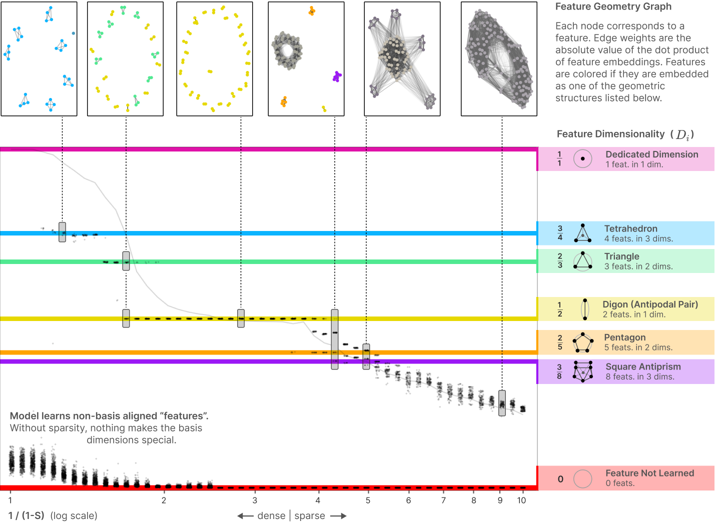


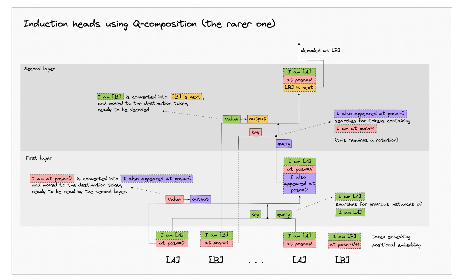
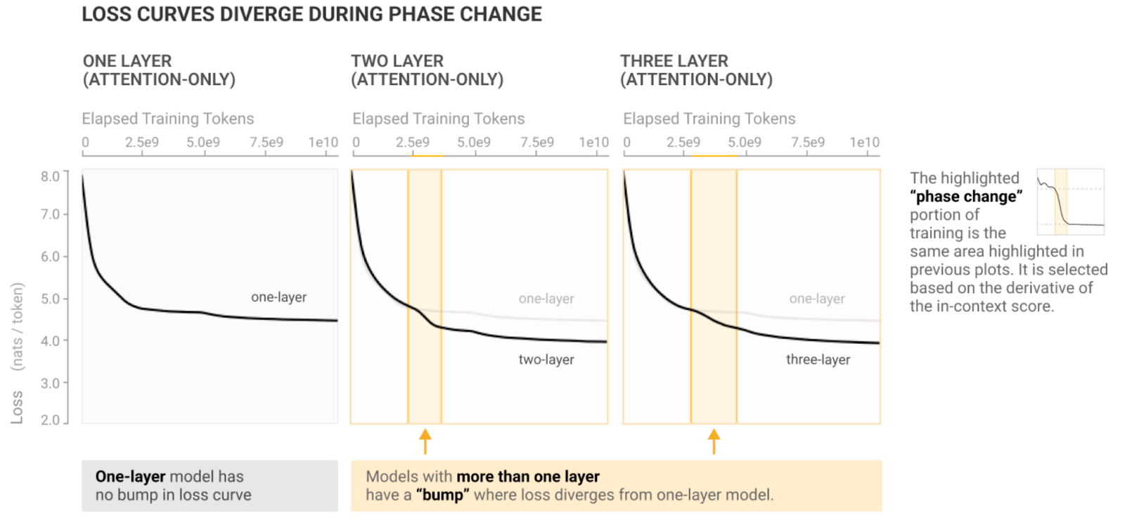


$\setCounter{0}$